3. B modeling

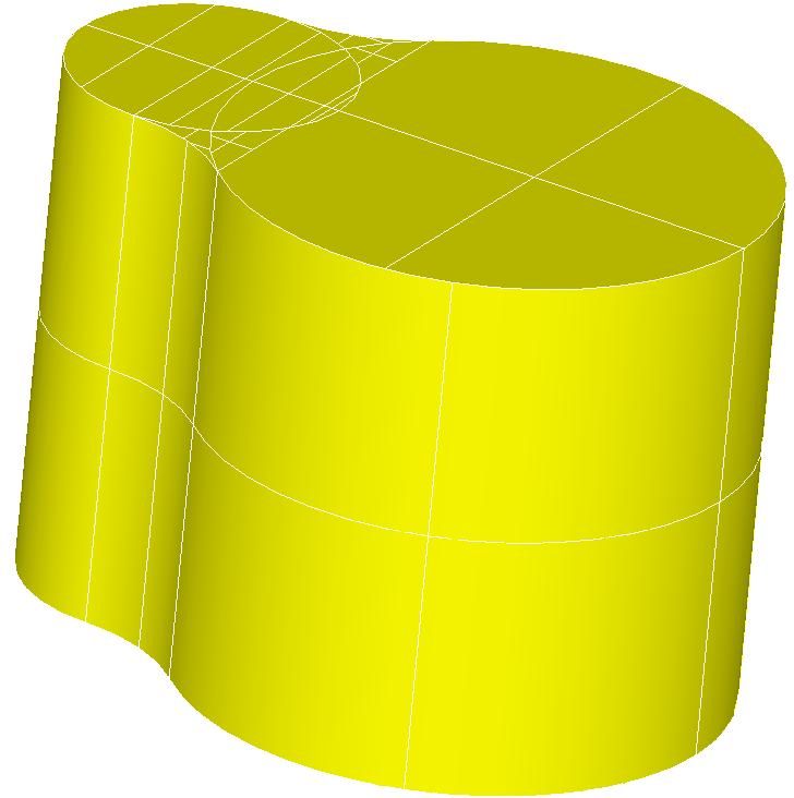
3.1. Geometry

3.2. Material properties

The material is the one defined for the test case of THM wtnl100a

3.3. Boundary conditions and loads

The calculation is in saturated hydromechanical nonlinear mechanics. After each adaptation, the calculation is initialized by the results of the previous calculation, interpolated on the new mesh. We will look at the evolution of the displacement on a node of the upper surface.

Face	Mechanics	Hydraulics
Higher	Imposed constraint	Zero flow
Lower	Zero displacement	Zero flow
Lateral	Zero Stress	Imposed Pressure

Mechanical problem:

The piece is stuck on the underside:

Side Z_ MIN: DX = DY = DZ = 0

Pressure is applied to the upper face:

Z_ MAX side: PRES = 1.0 105

The other edges have zero stress.

Hydraulic problem:

Pressure is applied to the lateral faces:

Faces COTE_0, COTE_1, * , COTE_2 , COTE_3 *: PRE1 = 1.0 105

The other edges have zero flow.

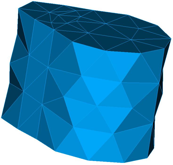
3.4. Characteristics of the mesh

The initial mesh before refinement.

Knots: 622

TRIA6: 148

TET10: 339

3.5. Benchmark results

DZ move for the node group A, consisting of a single node, after the 3rd adaptation:

DZ = -6.2381906050503x10-2

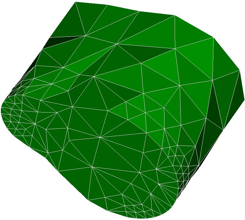
3.6. Adapted meshes

The Python mesh refinement loop includes 3 iterations starting from the jump of the mechanical displacement field from one node to its neighbor. For each iteration, the characteristics of each mesh produced by the macro-command MACR_ADAP_MAIL are described.

Knots: 1611

TRIA6: 362

TET10: 901

3.7. notes

We can see that the nodes resulting from the division of segments on the border will be placed on the analytical description of the border.

We will carefully look at the mechanism used to connect fields to Gauss points.