2. Modeling A#
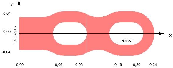
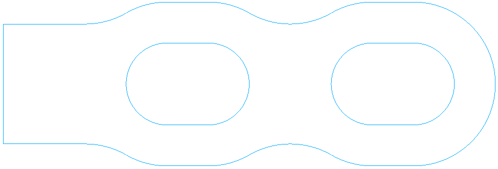
2.1. Geometry#
2.2. Material properties#
Material with elasto-plastic behavior with linear work hardening:
Elasticity:
\(E=2.1x{10}^{5}\mathrm{Pa}\) Young’s module
\(\nu =0.3\) Poisson’s ratio
Plasticity:
Slope of the traction curve in the plastic field \(\frac{\partial \sigma }{\partial \varepsilon }=2.\times {10}^{\mathrm{3 }}\mathrm{Pa}\)
Elastic limit \({\sigma }_{e}=235.\mathrm{Pa}\)
2.3. Boundary conditions and loads#
The calculation is in nonlinear mechanics. The piece is embedded on its left side. Pressure is exerted on the lower horizontal part of the second hole (zone \(\mathrm{PRES1}\) on the sketch). This pressure varies over time. We will look at the evolution of the displacement on a node of the base.
Edge ENCASTR: blocking movements by blocking degrees of freedom: DX = DY = 0.
Edge PRES1 loading
pressure imposed as a function of the moments:
Instant (s) |
Pressure (Pa) |
The other edges have zero stress.
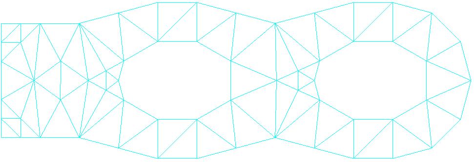
2.4. Characteristics of the mesh#
The initial mesh before refinement.
Knots: 158
SEG3: 45
TRIA6: 57
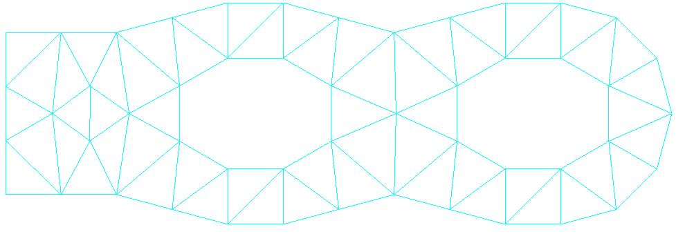
The discrete border is made up of 4643 knots and as many segments.
2.5. Benchmark results#
DX and DY movements for the node group A1, consisting of a single node, after the 3rd adaptation:
DX = -3.897029x10⁻⁵
DY = -1.395493x10⁻⁴
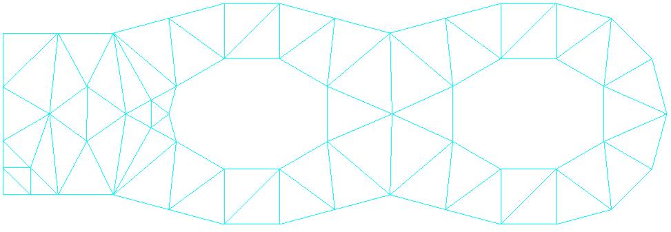
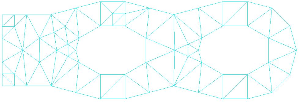
2.6. Adapted meshes#
The Python mesh refinement loop has 3 iterations starting from the error indicator (ERME_ELEM). For each iteration, the characteristics of each mesh produced by the macro-command MACR_ADAP_MAIL are described.
2.6.1. Refined mesh: iteration 1#
Knots: 179
SEG3: 48
TRIA6: 66
2.6.2. Refined mesh: iteration 2#
Knots: 200
SEG3: 51
TRIA6: 75
2.6.3. Refined mesh: iteration 3#
Knots: 219
SEG3: 52
TRIA6: 84
2.7. notes#
We can see that the nodes resulting from the division of segments on the border will be placed on the fine description of the border.