3. General presentation#
3.1. Principle of recalibration#
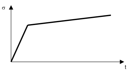
Let us consider the model problem of identifying the elastoplastic characteristics \(E\), \({\sigma }_{y}\), \({E}_{T}\) (respectively Young’s modulus, elastic limit and work hardening modulus) of a material on a uniaxial tensile test.
On the one hand, we have the experimental traction curve giving the evolution of the stress as a function of time and which is a data:
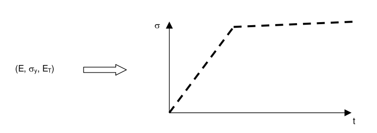
On the other hand, we have a function of the 3 parameters which for each value of the triplet \(E\), \({\sigma }_{y}\), \({E}_{T}\) returns a calculated traction curve:
The objective of the recalibration is then to answer the question:
What are the values of \((E,{\sigma }_{y},{E}_{T})\) that best describe my experience?
3.2. Organization of readjustment#
To carry out a successful registration, it is necessary to have all of the following information available:
the \(N\) experimental curves (to each of these curves can be assigned an arbitrary weight),
the \(P\) parameters to be adjusted as well as, for each, an estimate of its initial value, its minimum value and its maximum value,
the command file modeling the \(N\) tests you want to reset,
the names of the \(N\) quantities to be extracted from the command file above and which will be adjusted to the \(N\) experimental curves. These quantities must be contained in a table from POST_RELEVE_T.
Putting this information into data then requires the following organization:
a command file called**master* containing the \(N\) experimental curves, the \(P\) parameters, the names of the quantities to be adjusted as well as other information specific to the adjustment, all entered in MACR_RECAL. The various formats used are specified below,
a command file called**slave* modeling the experimental tests.
Indeed, resetting is a iterative process: the master file executes the slave file, it retrieves the \(N\) curves calculated with the current values of the \(P\) parameters, it compares the values of the calculated curves to those of the experimental curves, it deduces new values for the \(P\) parameters and relaunches the slave file. This process continues until convergence is achieved.
N experimental curves
Master file
MACR_RECAL
(study profile.com file)
P parameters
Recalibration loops
N calculated curves
Slave file
Figure 3.2-a. Diagram of the operation of the readjustment procedure for the classical case
The following section describes the operands of MACR_RECAL. It refers to some notions of the Python language. However, you do not need to know Python to use this macro command. The « Example of use » section is there to enlighten the user.
The data structure produced is a list of real numbers containing the values of the parameters at convergence in case of convergence or at the last iteration in the opposite case.
3.3. Special use case: fashion EXTERNE#
In this mode of use, the optimization algorithm is external to Code_Aster.
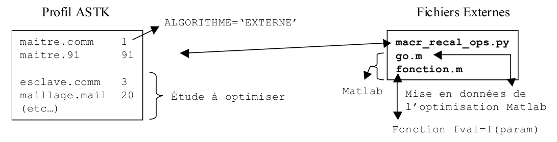
Figure 3.3-a : MACR_RECAL method EXTERNE
Code_Aster is just a black box that takes as input a text file containing the list of parameter values, performs the functional calculation for this set of parameters, possibly calculates the gradients with respect to the parameters, and returns to the external algorithm, via a text file, the value of the functional and possibly the gradients.
In this mode of operation, paragraph 3.1 remains valid.
3.4. Special case of realigning a dynamic model#
In the case of recalibrating the parameters of a dynamic model using experimental data from dynamic analysis, there are some particularities for the implementation. In this case, the experimental data are natural frequencies and eigenvectors (modal deformations) contained in a mode_meca concept resulting from the measurement.
The user has this concept using data acquisition software usually in « .unv » format and must build a so-called « experimental » model in order to use it in the Code_Aster environment. This « experimental » model contains, among other things, the experimental mesh, that is to say the mesh of the sensors, which is coarser than the mesh of the numerical model, which must also be available for the calibration study.
So the user no longer has to provide the experimental curves in the master file but he will enter here the names of the concepts that contain them, concepts that will be extracted by a first slave calculation from the external file « unv ». The format used to transmit this information to MACR_RECAL is the same as that for RESU_CALC: a Python list of \(N\) Python lists containing the names of the tables and columns containing the experimental answers.
Below is a diagram of the readjustment process in the case of dynamics:
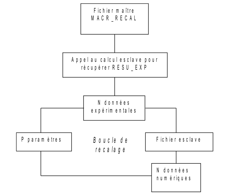
Figure 3.4-a. Diagram of operation of the dynamic readjustment procedure
Two other particularities concern the slave calculation command file:
it also contains the commands needed to build the experimental model. The mode_mecauusable concept for extracting RESU_EXP is provided by LIRE_RESU;
The quantities corresponding to the experimental and numerical answers are still contained in tables but no longer necessarily from POST_RELEVE_T. The responses related to modal deformations come either from CREA_TABLE (for the MAC experimental criterion), or from MAC_MODES (for the numerical MAC criterion). We recall that the criterion of MAC [U4.52.15] is used to compare two modal bases, here it is the experimental one and the numerical one.