4. Operands#
4.1. Operand UNITE_ESCL#
♦ UNITE_ESCL
Logical unit number of the slave file, assigned in the Astk interface (UL column). The extension of this file can be any.
4.2. Operands RESU_EXP, RESU_CALC, FONC_EXP, NOM_FONC_CALC,, PARA_X,, PARA_Y, POIDS#
The user has 2 input modes to fill in the experimental data and the names of the tables and columns of the calculated results.
He has the choice between using:
RESU_EXPet RESU_CALC and possibly LIST_POIDS which require Python lists to be entered,
the keywords FONC_EXP, NOM_FONC_CALC, PARA_X, PARA_Y, POIDSdu keyword factor COURBEqui have the advantage of using Aster concepts.
◊ RESU_EXP
Name of the Python list of \(N\) numpy arrays containing the \(N\) experimental curves. For a static model, the list is defined beforehand in the form:
resu_exp= [
    numpy.array ([[x0, y0], [x1, y1],... [xn, yn]])),
    ...
    numpy.array ([[u0, v0], [u0, v0], [u1, v1],... [one, vn]])
]
For the recalibration of a dynamic model with modal experimental data (frequencies and eigenvectors), this will be the name of the Python list of \(N\) Python lists containing the names of the tables and columns containing the experimental answers. For example:
resu_exp= [['REPEX1', 'NUM_ORDR', '', '', 'FREQ'], ['REPEX2', 'NUM_ORDR', 'MAC_EXP']]
◊ RESU_CALC
Name of the list of N Python lists containing the names of the tables and columns containing the numerical answers corresponding to the experimental measurements on which we will recalibrate. For example:
resu_calc= [['TABLE1', 'INST', '', '', 'SIYY'], ['TABLE2', 'INST', 'V1'],...]
◊ LIST_POIDS
Name of the Numpy array containing the \(N\) weights to be assigned to the \(N\) experimental curves. If the keyword is not entered, then each curve has the same weight. The list is defined beforehand in the form:
LIST_POIDS = numpy.array ([p1, p2,...])
◊ FONC_EXP
Name of the function previously defined by the DEFI_FONCTION operator that corresponds to the experimental data. To make the connection with RESU_EXP, the function provided to this keyword in iteration \(i\) corresponds to the \(i\) th numerical array of RESU_EXP.
   ◊ NOM_FONC_CALC

Character string corresponding to the name you want to assign to the function after resetting the experimental data.
   ◊ POIDS

Weight value to be assigned to the experimental curve. If not specified, then the value is 1.
   ◊ PARA_X

Name of the :math:`X` parameter for the calculated function.
   ◊ PARA_Y

Name of the :math:`Y` parameter for the calculated function. For example:
COURBE =(

_F (FONC_EXP =fct1, NOM_FONC_CALC =' TABLE1 ', PARA_X =' INST', PARA_Y =' SIYY ',),

_F (FONC_EXP =fct2, NOM_FONC_CALC =' TABLE2 ', PARA_X =' INST', PARA_Y ='V1',),)
4.3. Operands LIST_PARA, PARA_OPTI, NOM_PARA, VALE_INI,, VALE_MIN, VALE_MAX#
The user has 2 input modes to enter the names and values of the parameters.
He has the choice between using:
LISTE_PARA that require Python list entry,
the keywords NOM_PARA, VALE_INI, VALE_MIN, VALE_MAXdu keyword factor PARA_OPTI that have the advantage of using Code_Aster concepts (numerical values or character strings).
◊ LIST_PARA
Python list name of \(P\) Python lists containing variable names, initial values, minimum values, and maximum values. This list is defined beforehand in the form:
list_para= [['PARA1__', INI_1,, MIN_1, MAX_1],
    ['PARA2__', INI_2, MIN_2, MAX_2],
    ...
    ['PARAP__', INI_P, MIN_P, MAX_P]]
Attention:
Variable names are required to end in two underlined blanks (for example: YOUN__) .
Note:
The terminals are not managed by the FMIN, FMINBFGS and FMINNCG algorithms.
◊ NOM_PARA
Parameter name. The character string provided to NOM_PARAà iteration \(i\) corresponds to the first element of the \(i\) th python list in the list provided to LIST_PARA.
◊ VALE_INI
Initial value of the parameter. The real given to NOM_PARAà the iteration \(i\) corresponds to the second element of the \(i\) th python list in the list provided to LIST_PARA.
◊ VALE_MIN
Minimum value for the parameter. The real given to NOM_PARAà iteration \(i\) corresponds to the third element of the \(i\) th python list in the list provided to LIST_PARA.
◊ VALE_MAX
Maximum value of the parameter. The real given to NOM_PARAà iteration \(i\) corresponds to the fourth element of the \(i\) th python list in the list provided to LIST_PARA.
4.4. Operand UNITE_RESU#
◊ UNITE_RESU
Logical unit number of the readjustment result file (evolution of parameters during iterations, convergence criteria).
4.5. Operand ITER_MAXI#
◊ ITER_MAXI
Maximum number of readjustment iterations.
4.6. Operand ITER_FONC_MAXI#
◊ ITER_FONC_MAXI
Number of maximum functional evaluations.
4.7. Operand RESI_GLOB_RELA#
◊ RESI_GLOB_RELA
Relative overall residue of the recalibration.
This value is separate from the value specified for the nonlinear solvers STAT_NON_LINE and DYNA_NON_LINE.
4.8. Operand TOLE_FONC#
◊ TOLE_FONC
Criterion for stopping the readjustment algorithm based on the variation of the functional from one iteration to another. This criterion corresponds to the absolute value of the norm of functional MA.
4.9. Operand TOLE_PARA#
◊ TOLE_PARA
Criterion for stopping the readjustment algorithm based on the variation of parameters from one iteration to another. This criterion corresponds to standard \(\mathit{L2}\): the square root of the sum of the squares of the differences in each parameter.
4.10. Operand PARA_DIFF_FINI#
◊ PARA_DIFF_FINI
The adjustment requires the calculation of the derivatives of the responses with respect to the parameters.
This calculation is carried out by finite differences. PARA_DIFF_FINIES corresponds to \(\alpha\) in the following formula:
\(\frac{\mathrm{\partial }f}{\mathrm{\partial }x}\mathrm{\approx }\frac{f(x+\alpha x)\mathrm{-}f(x)}{\alpha x}\)
4.11. Operand GRAPHIQUE#
◊ UNITE
The logical unit number of the graphs produced during the realignment. At each iteration, MACR_RECAL produces \(N\) graphic files (whose format is defined by the keyword PILOTE) representing the \(N\) experimental and calculated curves.
◊ PILOTE
The type of graph display.
If PILOTE = “INTERACTIF” or “INTERACTIF_BG”, xmgrace is opened interactively with the chart. With “INTERACTIF_BG”, xmgrace is called in the background, the calculation continues.
If PILOTE is” POSTSCRIPT “,” EPS “,” MIF “,” “,” “,” SVG “,” “,” PNM “,” PNG “,” JPEG “, or” PDF “then xmgrace is used to generate the corresponding format file, in the logical unit defined by UNITE.
Attention:
Mode INTERACTIF is only possible when the readjustment is running interactively and not in batch.
◊ FORMAT
Choice of software for displaying curves in interactive mode: xmgrace or gnuplot. The use of Xmgrace is blocking: you must close the Xmgrace window to continue running.
◊ AFFICHAGE
Show curves at each iteration or only at the end.
4.12. Operand METHODE#
◊ METHODE
Optimization method or algorithm chosen:
LEVENBERG (default): Levenberg-Marquardt algorithm. This algorithm is the one recommended in quadratic minimization problems such as least squares, such as problems with the adjustment of material parameters.
FMIN: Nelder-Mead Simplex algorithm (only uses functional estimates).
FMINBFGS: Quasi-Newton method (uses the functional and the functional gradient).
FMINNCG: Newton Conjugate Gradient Line-search method (uses the functional, the functional gradient and the Hessian sound).
GENETIQUE: evolutionary algorithm based on the mechanism of selection and replacement. It is an algorithm that is expensive in time CPU, we recommend its use only for a rough exploration of the parameter space as part of the hybrid realignment technique presented in the next point.
HYBRIDE: technique that combines the stochastic with the deterministic - the evolutionary algorithm with the Levenberg—Marquardt algorithm
Mode EXTERNE: this method makes it possible to use an optimization algorithm external to Code_Aster, for example Matlab or Scilab, and to use Code_Aster only for the estimation of the functional and possibly of the gradient by finite differences. This is not a MACR_RECAL keyword because the EXTERNE mode is used directly by calling the bibpyt/Macro/recal.py file
Regarding the choice of the optimization algorithm, it is strongly recommended to opt for the algorithm by default, Levenberg-Marquardt. This is very often superior to the FMIN * algorithms for least squares minimization problems, such as parameter readjustment. Indeed, it uses the functional in its vector form while the other algorithms use a scalar functional, which is therefore less rich. In addition, it uses an active constraints method in order to manage limits on the parameters, while the other algorithms do not manage the limits.
The other algorithms can nevertheless be useful in cases where Levenberg-Marquardt is put in trouble. For example, algorithm FMIN does not use gradients, whose evaluation can in some very specific cases generate numerical problems (very sensitive parameters, too few experimental values, or others). Algorithm FMIN is much slower, but will be able to converge (to draw a parallel, the problem is similar to that of using the elastic matrix instead of the tangent matrix in STAT_NON_LINE).
For the Levenberg-Marquardt algorithm, the document [R4.03.06] describes more precisely the mathematical algorithm used.
The algorithms FMIN * were taken entirely from a Python module distributed on the Internet (http://pylab.sourceforge.net) () under license GPL by Travis E. Oliphant, who is also the main contributor to the Python-Scipy project and responsible for the Scipy optimization module. Algorithm and implementation details can be found on the page `http://pylab.sourceforge.net`_ < http://pylab.sourceforge.net/>.
Method HYBRIDE is recommended when there is a high degree of uncertainty about the optimal values of the parameters or when the functional has numerous local minima. Thus, in the framework of this method, we first launch a rough search with the evolutionary algorithm, which will make it possible to avoid local minima, followed by refining the optimization with the Levenberg-Marquardt algorithm.
4.13. Keyword CALCUL_ESCLAVE#
4.13.1. Operand LANCEMENT#
◊ LANCEMENT
Method for launching slave files: inclusion or distribution. Both modes have advantages and disadvantages and the choice of one or the other depends mainly on the calculation times of the slave files, as well as on their compatibility with Inclusion mode.
4.13.2. Operand INCLUSION#
◊ INCLUSION

In this mode, the slave file is included. There is therefore no waste of time in generating a new study, creating the temporary execution directory, etc. On the other hand, only a slave study will be able to pass on the machine at the same time. On the other hand, some slave studies (for example those using embedded data files, or slightly complex execution profiles) are not compatible.
Note:
In mode INCLUSION, the Aster INCLUDE command cannot be present in the slave file (incompatibility with the Aster supervisor) .
The command must therefore be replaced:
INCLUDE (UNITE =n)
by the order:
execfile (fort.n)
where n is the logical unit of the file to include.
4.13.3. Operand DISTRIBUTION, MODE, MEMOIRE, TEMPS,, CLASSE, UNITE_SUIVI#
◊ DISTRIBUTION

In this mode, at each iteration of the optimization algorithm, the :math:`N+1` slave calculations (for a recalibration of :math:`N` parameters) are executed in parallel, in batch or interactively, using the as_run distributed calculation module. Compared to Inclusion mode, each study takes slightly longer to run, because you have to regenerate a new Code_Aster study, create temporary files, etc. On the other hand, as the studies are launched in parallel, according to the characteristics of the slave studies (size and duration), the greater the number of parameters, the more the Distributed mode becomes more interesting than the Inclusion mode.


In distributed mode, additional parameters are available to control the execution of slave calculations:
◊ MODE: INTERACTIF or BATCH
◊ MEMOIRE: memory in MB
◊ TEMPS: time in seconds
◊ CLASSE: batch class, allows you to force calculations to use a specific class, for example "distr" on the Code_Aster server
◊ UNITE_SUIVI: if this keyword is specified, it defines the logical unit of the profile file in which all the output files of the slave jobs will be stored
◊ NMAX_SIMULT: number of slave calculations started in parallel in distribution mode (if no value is entered, the code automatically decides on this number)


It is possible to use parallelism MPI for slave studies. In this case, it is necessary to launch the master calculation with version MPI and on a single processor (in interactive mode or in batch). The MPI characteristics of slave calculations should be indicated by the following keywords:
◊ MPI_NBCPU: number of processors MPI for each of the slave calculations started in parallel
◊ MPI_NBNOEUD: number of nodes for each slave calculation started in parallel


Note that operational problems may interfere with the launch of distributed slave calculations (for example, batch classes are poorly defined and calculations cannot be executed). In this case, the error obtained in the master computation .mess can be quite simple (an error message like "at least one of the slave calculations could not start"). To get additional information about the distributed as_run module, you must simultaneously set UNITE_SUIVI and INFO =2.
4.14. Operands NB_PARENTS and NB_FILS#
◊ NB_PARENTS
For the GENETIQUE or HYBRIDE method, this operand defines the size of the parameterized population. Initially all individuals are identical and initialized with the initial values of the parameters provided by the user in LIST_PARA. During optimization the population evolves, the less « adapted » individuals being replaced by others who provided better functional value.
◊ NB_FILS
Represents the population replacement rate. More exactly, the best « parent » (the one for which the value of the functional is minimal) has the right to reproduce thus generating NB_FILS « son ». At this time the population size is NB_PARENTS + NB_FILS. According to the hierarchy of functional values, only the best individuals from all this population are retained and we return to the initial size: NB_PARENTS.
4.15. Operand ECART_TYPE#
◊ ECART_TYPE
This is the value of the standard deviation that the user imposes for the semi-random draws of the « threads ». The more you want to explore the topological space of the parameters, the more you need to increase this value. Corroborated to the size of the population and the replacement rate, this operant makes it possible to control the evolutionary algorithm according to the complexity of the model and the degree of uncertainty about the optimal values of the parameters. If little is known about the values of the parameters to be adjusted, it is recommended to use a large population size, an equally high replacement rate and a large standard deviation. The payback will be a very high CPU time.
4.16. Operand ITER_ALGO_GENE#
◊ ITER_ALGO_GENE
Maximum number of iterations for the evolutionary algorithm. If we use the HYBRIDE method, this value (or RESI_ALGO_GENE) will determine the transition to the Levenberg-Marquardt algorithm.
4.17. Operand RESI_ALGO_GENE#
◊ RESI_ALGO_GENE
Relative residue of the recalibration of the evolutionary algorithm. If we use the HYBRIDE method, this value (or ITER_ALGO_GENE) will determine the transition to the Levenberg-Marquardt algorithm.
4.18. Operand GRAINE#
◊ GRAINE
Value imposed by the user for the seed of the random draw generator in the evolutionary algorithm. If we enter a value for this keyword, we force the random number generator present in the evolutionary algorithm to always generate the same draws, so we will have a repetition of the solution. Its use is reserved only for test cases for reasons of monitoring the non-regression of the code.
4.19. Operand DYNAMIQUE#
This operand is entered in order to recalibrate the parameters of a dynamic model by modal analysis.
◊ MODE_EXP
Name of the mode_meca concept that contains experimental modal data. This concept is extracted in the slave calculation by a LIRE_RESU.
◊ MODE_CALC
The name of the mode_meca concept that contains numerical modal data. This concept is calculated in the slave file by a CALC_MODES.
◊ APPARIEMENT_MANUEL
Choice to display a graphical window in interactive mode that will allow the specific modes to be mapped manually. For example, the incorrect automatic pairing of double-crossed natural modes is thus avoided.
The screenshot shown in Figure 4.19-a shows this graphical window.
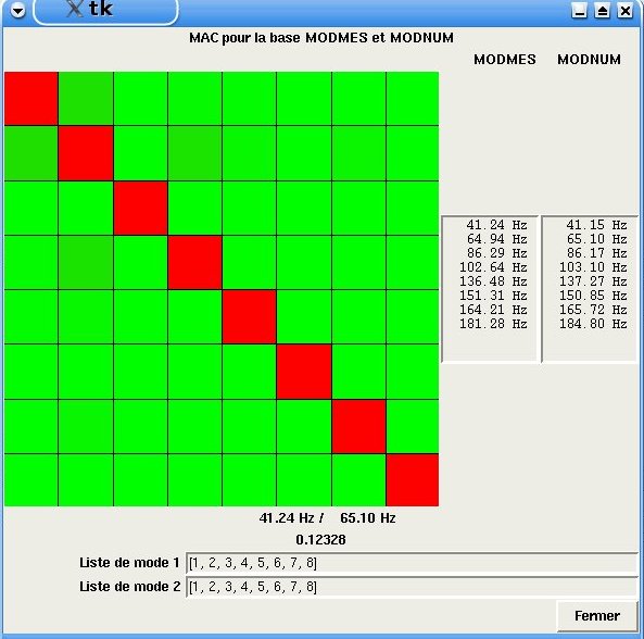
Figure 4.19-a. Graphic window for the manual pairing of MAC
The user thus sees, at each generation of the evolutionary algorithm or at each iteration of the Levenberg-Marquardt algorithm, the MAC matrix and can decide to change the pairing by modifying the order of the modes in the lists located at the bottom of the window. This window is blocking the execution of Code_Aster commands so it must be closed for the recalibration process to continue. Closing the window by clicking on the Close button allows you to retrieve the new lists of modes whose order may have been modified by the user.
4.20. Operand GRADIENT#
◊ GRADIENT
For methods FMINBFGS, FMINNCG or EXTERNE, this keyword allows you to tell Code_Aster how to calculate the gradients (undimensioned or not), or not to step them.
Note: for algorithms that use gradients, they can be calculated by differences automatically finite by Code_Aster, or calculated in the slave file using, for example, sensitivity calculations (keyword LIST_DERIV).