6. Examples of use#
6.1. Identification of the parameters of an elastoplastic behavior law on a tensile test#
This example is covered by test ZZZZ159A [V1.01.159].
6.1.1. Problem position#
The results of a tensile test are available. This is the evolution of stress \({\sigma }_{\mathrm{yy}}\) over time as well as the evolution of the cumulative plastic deformation \(p\) over time.
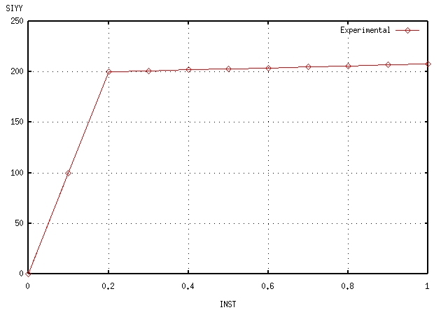
Constraint SIYY |
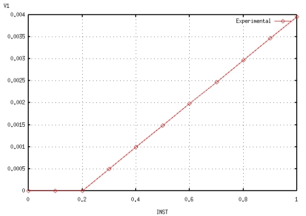
Cumulative plastic deformation |
It is desired to adapt the Young’s modulus, the yield strength and the work-hardening slope of an elastoplastic behavior law with linear isotropic work hardening to these tests.
6.1.2. Data setting#
6.1.2.1. Experiment#
First of all, we start by defining our test results. They consist of two curves that are defined as follows.
exper1 = DEFI_FONCTION (
     NOM_PARA =' INST ',
     NOM_RESU =' SIYY ',
     VALE =( 0.00000E+00, 0.00000E+00,
     5.00000E-02, 5.00000E+01,
     ...
     9.50000E-01, 2.07500E+02,
     1.00000E+00, 2.08000E+02),)

exper2 = DEFI_FONCTION (
     NOM_PARA =' INST ',
     NOM_RESU ='V1',
     VALE =( 0.00000E+00, 0.00000E+00,
     5.00000E-02, 0.00000E+00,
     ...
     9.50000E-01, 3.71250E-03,
     1.00000E+00, 3.96000E-03),)
exper1 and exper2 are therefore functions that represent stress \({\sigma }_{\mathrm{yy}}\) and cumulative plastic deformation \(p\) respectively.
6.1.2.2. Calculus#
We then write the Code_Aster slave command file modeling this traction test where our 3 parameters and the two curves to be adjusted will appear.
DEBUT ()

# AFFECTATION DES VALEURS DES PARAMETRES A RECALER
# LES VALEURS RENSEIGNEES ICI SONT SANS IMPORTANCE
# SEULES COMPTENT LES VALEURS RENSEIGNEES DANS THE FICHIER MAITRE
DSDE__ = 200.
YOUN__ = 8.E4
SIGY__ = 1.

ACIER = DEFI_MATERIAU (
     ECRO_LINE =_F (
          D_ SIGM_EPSI = DSDE__,
          SY= SIGY__,),
     ELAS =_F (
          NU=0.3,
          E= YOUN__,),)
...

U= SIMU_POINT_MAT (
     COMPORTEMENT =_F (RELATION =' VMIS_ISOT_LINE '),
     MATER = ACIER,
     INCREMENT =_F (LIST_INST = INSTANTS,),
     NEWTON =_F (REAC_ITER =1),
     EPSI_IMPOSE =_F (EPYY =epyy,),
)

EXTRACTION OF THE REPONSE SIGMAYY (T)
REPONSE1 = CALC_TABLE (
     TABLE = U,
     ACTION =_F (OPERATION =' EXTR ',
     NOM_PARA =( 'INST', 'SIYY', ''))

EXTRACTION OF THE REPONSE EPSP (T)
REPONSE2 = CALC_TABLE (
     TABLE = U,
     ACTION =_F (OPERATION =' EXTR ',
     NOM_PARA =( 'INST', 'V1')))

FIN ()
6.1.2.3. MACR_RECAL#
We now need to define in the master file the initial values and the ranges of variations of our parameters. We want to:
1.E5 < Initial Young's Modulus = 1.E5 < 5.E5
5. < Initial elastic limit = 30. < 500
1.E3 < Initial work hardening module = 1.E3 < 1.E4
Finally, it is also necessary to define in the master file the quantities to be extracted from the slave command file. On the one hand, we want to extract column INST and column SIYY from table REPONSE1 and on the other hand column INST and column V1 from table REPONSE2. We write it:
Here’s how we fill in this information in the body of MACR_RECAL:
RESU2 = MACR_RECAL (
    UNITE_ESCL =3,
    PARA_OPTI =(
        _F (NOM_PARA =" YOUN__ ", VALE_INI =100000.0, =100000.0, VALE_MIN =50000.0, VALE_MAX =500000.0),
        _F (NOM_PARA =" DSDE__ ", VALE_INI =1000.0, VALE_MIN =500.0, VALE_MAX =10000.0),
        _F (NOM_PARA =" SIGY__ ", VALE_INI =30.0, =30.0, VALE_MIN =5.0, VALE_MAX =500.0),
    ),
    COURBE =(
        _F (FONC_EXP =exper1, NOM_FONC_CALC =" REPONSE1 ", PARA_X =" INST ", PARA_Y =" SIYY "),
        _F (FONC_EXP =exper2, NOM_FONC_CALC =" REPONSE2 ", PARA_X =" INST ", PARA_Y ="V1"),
    ),
)
6.1.2.4. Alternative data layout (Python lists)#
You can use Python list-based and numpy object-based data layout. The master file will then be written:
experience = [
numpy.array (
     [
          [0.00000e00, 0.00000e00],
          [5.00000e-02, 5.00000e01],
          ...
          [9.50000e-01, 2.07500e02],
          [1.00000e00, 2.08000e02],
     ]
),
numpy.array (
     [
          [0.00000e00, 0.00000e00],
          [5.00000e-02, 0.00000e00],
          ...
          [9.50000e-01, 3.71250e-03],
          [1.00000e00, 3.96000e-03],
     ]
),
]

parameters = [
[" YOUN__ ", 100000.0, 50000.0, 500000.0],
[" DSDE__ ", 1000.0, 500.0, 10000.0], 10000.0],
[" SIGY__ ", 30.0, 5.0, 500.0],
]

calculation = [[" REPONSE1 "," INST "," "," SIYY "]," "], [" REPONSE2 "," INST ", "V1"]]
where: experience is the name of a Python list (defined in square brackets) of 2 numpy arrays, parameters is a list of Python lists containing the initial values and ranges of variations of our parameters and*calculate* the quantities to be extracted from the slave command file.
The body of the command is then written:
RESU = MACR_RECAL (UNITE_ESCL =3, RESU_EXP =experience, LIST_PARA =parameters, RESU_CALC =calculation)
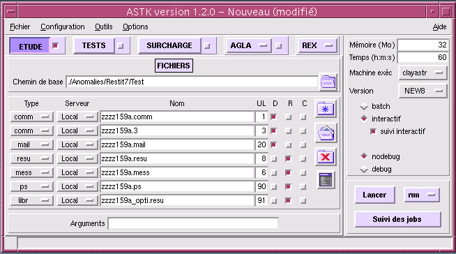
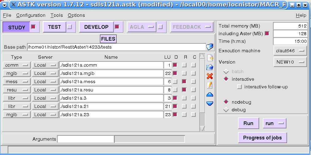
6.1.2.5. Astk#
Finally, the following study profile is defined:
6.1.3. Results#
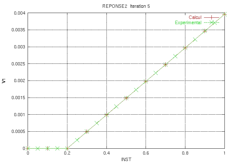
Once the study has been completed, the ZZZZ159_opti .resu calibration result file contains the following information:
Calculating sensitivity with respect to = YOUN__ DSDE__ SIGY__

======= =====

Iteration 0 =

=> Functional = 1.0

=> Residue = 1.0

=> Parameters =

YOUN__ = 100000.0

DSDE__ = 1000.0

SIGY__ = 30.0

======= =====

Calculating sensitivity with respect to = YOUN__ DSDE__ SIGY__

======= =====

Iteration 1 =

=> Functional = 0.259742161795

=> Residue = 0.30865397471

=> Parameters =

YOUN__ = 300857.888503

DSDE__ = 9135.12770111

SIGY__ = 152.548047532

======= =====

Calculating sensitivity with respect to = YOUN__ DSDE__ SIGY__

======= =====

Iteration 2 =

=> Functional = 0.0757636994765

=> Residue = 0.473053125246

=> Parameters =

YOUN__ = 157723.378846

DSDE__ = 2022.7431335

SIGY__ = 213.155325073

======= =====

Calculating sensitivity with respect to = YOUN__ DSDE__ SIGY__

===== ===== =====

Iteration 3 =

=> Functional = 0.00190706595529

=> Residue = 0.0520849911718

=> Parameters =

YOUN__ = 192302.166747

DSDE__ = 895.845518907

SIGY__ = 203.753909707

===== ===== =====

Calculating sensitivity with respect to = YOUN__ DSDE__ SIGY__

===== ===== =====

Iteration 4 =

=> Functional = 2.70165453323e-06

=> Residue = 0.00172172540305

=> Parameters =

YOUN__ = 199801.572817

DSDE__ = 1928.08902726

SIGY__ = 200.274590793

===== ===== =====

Calculating sensitivity with respect to = YOUN__ DSDE__ SIGY__

===== ===== =====

Iteration 5 =

=> Functional = 2.65431115925e-12

=> Residue = 1.83121468206e-06

=> Parameters =

YOUN__ = 199999.975047

DSDE__ = 1999.86955101

SIGY__ = 200.000462987

===== ===== =====

===== ===== =====

CONVERGENCE ATTEINTE

===== ===== =====

Hessian eigenvalues:

[7.17223479e+00 3.67264061e-01 6.25194340e-04]

Associated eigenvectors:

[0.98093218 -0.00549396 -0.19427266]

[-0.19418112 -0.06940835 -0.97850712]

[0.00810827 -0.9975732 0.0691517]
We can to derive/to establish that:
The following combinations of parameters are important for your calculation:
associated with the eigenvalue 7.2E+00
The following combinations of parameters are insensitive for your calculation:
associated with the eigenvalue 6.3E-04
And the POSTSCRIPT ZZZZ159 .ps file contains:
|
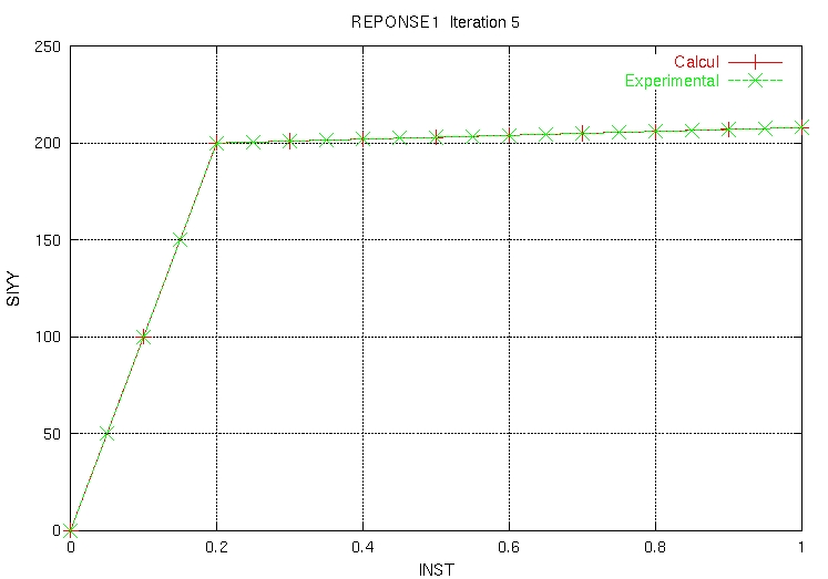
|
6.2. Identification of the parameters of a dynamic model by exploiting the sensitivity of natural modes#
This example is covered by test SDLS121A [V2.03.121].
We want to recalibrate the thickness of a plate and the value of a discrete mass that is located on it by using experimental natural mode measurements.
6.2.1. Data setting#
In the master file, you first enter the names of the tables that will contain both the calculated results and the numerical results:
calculation = [[" REPONSE1 "," NUME_ORDRE "," "," FREQ "]," "], [" REPONSE2 "," NUME_ORDRE "," MAC "]]

experience = [[" REPEXP1 "," NUME_ORDRE "," "," FREQ "]," "], [" REPEXP2 "," NUME_ORDRE "," MAC_EXP "]]
It is important to note here that, for the calculated results, the REPONSES2 is given by the diagonal of the MAC matrix from the MAC_MODES command as we will see later in this paragraph. The name of the parameter “MAC” is therefore a reserved name, chosen in this way in Fortran, and therefore it can no longer be used later (for the corresponding experimental answer we chose “MAC_EXP”)
The options used in command MACR_RECAL, still in the master file, are:
RESU = MACR_RECAL (
     UNITE_ESCL =3,
     RESU_EXP =experience,
     LIST_PARA =parameters,
     RESU_CALC =calculation,
     POIDS =weight,
     METHODE =" HYBRIDE ",
     ITER_FONC_MAXI =500,
     NB_PARENTS =10,
     NB_FILS =5,
     ECART_TYPE =10.0,
     ITER_ALGO_GENE =2,
     DYNAMIQUE =_F (MODE_EXP =" MODMES ", MODE_CALC =" =" MODNUM ", APPARIEMENT_MANUEL =" NON "),
)
We therefore chose to launch the realignment using method HYBRIDE with two iterations for the evolutionary algorithm. Finally, the following profile for the study is defined:
6.2.2. Slave calculation#
The main particularity of slave calculation is the presence in the command file (unit 3) of two models: the experimental model and the numerical model. Below is presented, for this test case, the slave command file with the necessary explanations.
reading the experimental mesh (the sensor mesh):
creation of a group of nodes that will later be used to define a discrete mass element:
creation of the group of nodes to define the boundary conditions:
creation of a POI1 element to introduce discrete mass:
assignment of the experimental model:
definition of elementary characteristics, material, etc.
CAREXP = AFFE_CARA_ELEM (...)

ACIER = DEFI_MATERIAU (...)

MATEX = AFFE_MATERIAU (...)
elementary calculations and matrix assemblies.
KELEXP = CALC_MATR_ELEM (OPTION =' RIGI_MECA ',
...)

MELEXP = CALC_MATR_ELEM (OPTION =' MASS_MECA ',
...)

NUMEXP = NUME_DDL (...)

KASSEXP = ASSE_MATRICE (...)

MASSEXP = ASSE_MATRICE (...)
creation of the sd_mode_meca with experimental eigenmodes:
And we continue with the numerical model, the same steps. The parameters to be adjusted are « EP__ » (the thickness) and « MP__ » (the mass):
EP__ = 0.5
MP__ = 50000.0
PRE_GIBI (UNITE_GIBI =22)

# number of frequencies
NF = 8

MODES = CALC_MODES (
     MATR_RIGI =M_ AS_RIG,
     MATR_MASS =M_ AS_MAS,
     OPTION =" PLUS_PETITE ",
     CALC_FREQ =_F (NMAX_FREQ =NF),
     SOLVEUR_MODAL =_F (METHODE =" SORENSEN "),
     VERI_MODE =_F (STOP_ERREUR =" NON "),
)
The experimental mesh is always coarser than the numerical model mesh, so it is necessary to project the numerical result onto the experimental mesh:
MODNUM = PROJ_CHAMP (RESULTAT = MODES, MODELE_1 = MODEL, MODELE_2 = MODEXP, NUME_DDL = NUMEXP)
The table of experimental frequencies is recovered.
REPEXP1 = RECU_TABLE (CO= MODMES, NOM_PARA =" FREQ ")
We are building the table of MAC experimentals - in fact the ideal MAC which is 1.0
mac_list = [1.0] * NF

REPEXP2 = CREA_TABLE (
     LISTE =( _F (PARA =" NUME_ORDRE ", LISTE_I =range (1, NF + 1)), _F (PARA =" MAC_EXP ", LISTE_R =mac_list))
)
And finally the tables with the calculated answers:
REPONSE1 = RECU_TABLE (CO= MODES, NOM_PARA =" FREQ ")

REPONSE2 = MAC_MODES (BASE_1 = MODNUM, BASE_2 = MODMES)
The results (the adjusted values of the parameters) are then calculated in a similar way with the classical case of readjustment presented in the preceding paragraph.
6.3. Parametric identification of a conservative system by exploiting the orthogonality of natural modes#
This example is treated by the D modeling of test case SDLS121 [V2.03.121].
We want to recalibrate the thickness of a plate and the value of a discrete mass that is located on it by using experimental natural mode measurements.
On the basis of the modal deformations noted at the observation points, an expansion is carried out on the support numerical model. We then try to find the parameters of the model such that the generalized mass and stiffness matrices relating to the modes identified experimentally are diagonal and that the difference between the measured natural pulsation and the calculated natural pulsation is minimal.
6.3.1. Data setting#
The technique, illustrated here, uses the modal deformations identified extended to the supporting numerical model. This modal deformation can be obtained using an independent calculation by depositing the extended deformations into a file that will be read later by the slave file. For practical reasons, the expansion is performed in the pilot file. This makes it easier to retrieve the support model that will be used in the slave file.
In the master file, both the target values (experimental values) and the names of the tables containing the results obtained from the numerical calculation performed in the slave file are entered.
The various steps are recalled below.
Creation of an experimental model in order to be able to define the location of the measurement points. The nodes of the mesh can be linked together by discrete elements to facilitate the visualization of the measured information. The mechanical characteristics that are assigned to this model do not affect the results, they allow the model to accommodate the identified natural modes
Reading the identified clean modes
Creation of the digital model to support the expansion of the measurement
Definition of the expansion base (here, a modal basis)
Calculation of the coordinates of the modes identified in the expansion base
Expansion of the information measured on the support model
Writing extended modes to a file in order to be able to use it in slave calculation
Definition of target values
The target values are stored in two lists. The first list contains extra-diagonal terms that should be zero and the second list contains the identified natural frequencies.
Definition of readjustment parameters
Launch of the optimization procedure
6.3.2. Slave calculation#
The slave calculation creates tables that will contain the values calculated from the input parameters. The various calculation steps are described below:
Creation of the support model (same DDL numbering as that used to expand the measure)
Reading extended modal deformations
Calculation of generalized mass and stiffness matrices via MAC_MODES
Creation of tables that contain the extradiagonal terms of the generalized matrices
Creation of the table containing the natural frequencies estimated using generalized matrices
6.4. Parametric identification of a dissipative system by exploiting the norm relationships of modal deformations#
This example is treated by modeling E from test case SDLS121 [V2.03.121].
We want to recalibrate the thickness of a plate, the value of a point mass on the plate and the discrete dampments distributed on the plate.
From the complex modal deformations identified at the observation points, an expansion is carried out on the support numerical model. We then try to find the parameters of the model in such a way that the eigenmodes identified experimentally verify the norm relationships associated with the numerical model. We focus only on the diagonal terms of the normalization matrix.
6.4.1. Data setting#
The data layout is similar to that presented in the previous chapter (6.3). The difference lies in the expansion of the modal deform. The modal deformations are complex here. The expansion is carried out by treating the real part and the imaginary part independently. The extended complex deformation is obtained after assembling the real deformation and the imaginary extended deformation.
The various steps are described below:
Creation of the experimental model
Reading the identified eigenmodes (experimental)
Expansion of the measure
Definition of target values (the target values are zero vectors here)
Definition of readjustment parameters
Launch of the optimization procedure
6.4.2. Slave calculation#
The slave calculation creates the tables that will contain the diagonal terms of the normalization matrix.
The various calculation steps are described below:
Creation of the support model (same DDL numbering as that used to expand the measure)
Reading extended modal deformations
Reading of natural frequencies and reduced damping
Calculating matrix products vector by PROD_MATR_CHAM
creation of the table that contains the terms relating to depreciation and mass: \(\frac{{y}_{\nu }^{T}B\stackrel{̄}{{y}_{\nu }}+2\Re ({s}_{\nu }){y}_{\nu }^{T}M\stackrel{̄}{{y}_{\nu }}}{\mid {n}_{\nu }\mid }={z}_{1\nu }\)
creation of the table that contains the terms relating to stiffness and mass: \(\frac{{s}_{\nu }\stackrel{̄}{{s}_{\nu }}{y}_{\nu }^{T}M\stackrel{̄}{{y}_{\nu }}-{y}_{\nu }^{T}K\stackrel{̄}{{y}_{\nu }}}{\mid {n}_{\nu }{s}_{\nu }\mid }={z}_{2\nu }\)
creation of the table that contains the terms relating to mass, stiffness and damping: \(\frac{{s}_{\nu }^{2}{y}_{\nu }^{T}{\mathit{My}}_{\nu }+{s}_{\nu }{y}_{\nu }^{T}{\mathit{By}}_{\nu }+{y}_{\nu }^{T}{\mathit{Ky}}_{\nu }}{{n}_{\nu }{s}_{\nu }}={z}_{3\nu }\)