2. How parametric calculations work#
2.1. Principle#
Implementing parametric studies in*Code_Aster* is relatively easy. However, it is important that:
your standard study runs smoothly before undertaking this type of calculation.
you have clearly defined in advance the parameters you want to vary:
their names,
their values,
the calculation scenarios to be executed.
In the case of a standard study you have at least:
In data:
of a command file (.comm)
the necessary data files (.mail, .med,…)
parameters (time and memory)
Out:
of a message file (.mess)
of a result file (.resu, .med,…)
To perform a parametric study you also need:
In data:
a file describing the parameter set (.distr)
from a results directory (.repe)
of an Astk distrib=yes option. Depending on the server, you may need to specify the batch class in which the calculations will be submitted.
the parameters (time/memory) are the same for all calculations, those of the master job can be set independently of the study by the plugin mechanism (cf. [U1.04.00]).
Out:
from a results directory (.repe)
In the following paragraphs we go over all these points in detail.
In the following table we have summarized the mandatory and optional elements that are found in the case of a parametric study.
Table 2.1-1: Summary of mandatory and optional elements in a parametric study
2.2. Implementation#
The actions to be taken to implement a parametric calculation are as follows:
Writing a set of parameters,
Use of parameters in the command file,
Under Astk tab ETUDE: defining the results directory and adding the parameter set,
Under Astk menu OUTILS: definition of the type of calculation
2.2.1. Writing a parameter set#
The description, in Python language, of the set of parameters is given in the file “.distr”. in which we find
the list of parameters,
the values that these parameters will take successively (calculation scenarios).
Example:
# young, temp_impo: variable names

# the variable young will have values 2.1E11 and 7.E10

# the temp_impo variable will have values of 100 and 273

VALE =(

_F (young=2.1E11, temp_impo = 100.), # calculation scenario 1


_F (young=7.0E10, temp_impo = 273.), # calculation scenario #2

)
Figure 2.2.1-a: Example of an explicit « distr » file
In this example, we have two calculation scenarios (No. 1 and No. 2) with the parameters young and temp_impo which will take \((2.1E11,100)\) and \((7.0E10,273)\) as values in succession.
At this stage, although the names of the parameters are sufficiently explicit, there is no way to say how they will be used. For the young parameter, this suggests that this one will be used when defining the material, but at the moment there is nothing to confirm this.
From a Python language point of view, the “.distr” file contains a list of dictionaries with the name VALE, (each dictionary corresponding to a calculation). We use _F as in the command file to define these dictionaries.
The definition of the parameters of the calculation scenarios can be given explicitly or calculated.
Note
In the previous example, the definition of the parameters and the calculation scenarios are given explicitly. It is possible to use the functionalities of the Python language to define them automatically, a practical example is presented in § 3.2.2 ) .The name of the parameters is defined by the user, it is recommended to use explicit names.
2.2.2. Using parameters in the command file#
In paragraph § 2.2.1, we defined the set of parameters (name, values and calculation scenarios), the objective now is to use these parameters in the command file, at the desired location.
These parameters are taken into account in the command file in two stages:
declaration of Python variables: the parameters
use of these variables in the command file.
Declaring parameters (python variables)
Before any use in a command or in any expression, it is required that the parameters are known. The aim is not to initialize them again, but simply to declare them as Python variables.
Example: in the previous.distr file, we defined the parameters young and temp_impo. The following lines will therefore be found in the command file:
DEBUT ()

...

young = 0.

temp_impo = 0.

...

FIN ()
Figure 2.2.2-a: Parameter declaration
Notes:
The values assigned in the command file will not be used, they will be automatically replaced by those defined in the file “distr”, for each calculation scenario.
Avoid choosing a parameter name that is the same as a Code_Aster keyword. Since the substitution is made by the regular expression “^ (*) name*=*”, there could be confusion.*Since case is significant, using lowercase names helps to avoid this pitfall. *
Using settings
The parameters in the command file are used in a conventional manner, within commands, mathematical expressions,…
Example:
DEBUT ()

...

young=0.

temp_imp=0.

...

mat= DEFI_MATERIAU (ELAS =_F (E=young,...))

...

t0 = AFFE_CHAR_CINE =( THER_IMPO =_F (TEMP =temp_impo,

GROUP_NO =' CHAUD ',..)

...


FIN ()
Figure 2.2.2-b. : Command file
2.2.3. Parameter type#
The type of parameters can be any. Next, keep in mind that the replacement is textual when instantiating the command set for a given set of parameters.
Example:
Let’s say the set of parameters:
VALE =( _F (young = 2.1e11, index = 4, noun = « “INST” », object = “FON1”,),),…)
and the command set header:
young = 2.e11index = 0nomp = “x’objf = FON0…
The command set based on the parameter set will be:
young = 2.1e11index = 4nomp = “INST “objf = FON1…
The difference is visible for the last two parameters where we see that we used the text of the character string of nomp and objf (and not the representation of this one, so a set of dimensions/quotes has disappeared).
This makes it possible to parameterize the use of concepts. Here, we use the FON1 function as the objf parameter.
2.2.4. File type settings#
In cases where the variable parameter is a file (for example to read a different mesh), it is a question of making the name of this file variable (text string or file number) and using DEFI_FICHIER.
Example that mixes a file name into a string and the same thing using a mesh number:
Let’s say the set of parameters:
VALE =( _F (fname = « ”/tmp/mesh_01.mmed” », index = 1,), _F (fname = « ”/tmp/mesh_02.mmed” », subscript = 2,),…)
and the command file:
fname = “filename_med’index = 0# using file name DEFI_FICHIER (ACTION =” ASSOCIER “, UNITE =20, FICHIER =fname) mesHa = LIRE_MAILLAGE (FORMAT =” MED”, UNITE =20) # using a file index (we build the file name# from the index on 2 characters # with 0s in front) filename = “/tmp/mesh_ {i:0>2} .mmed”.format (i=index) DEFI_FICHIER (ACTION =” ASSOCIER “, UNITE =21, FICHIER =21, =filename) MeshB = LIRE_MAILLAGE (FORMAT =” MED”, UNITE =21)
2.3. Launch of studies: Astk#
The launch of parametric studies is managed directly by Astk. This launch is identical to that of a traditional study with the addition of additional information such as:
addition of a line to the study profile to take into account the “distr” file
addition of a line to the study profile to define the “repe” result directory
initialization in the option menu, of the distrib parameter to “OUI”.
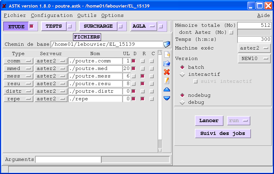
Figure 2.3-a : Parameter set definition, directory (astk)
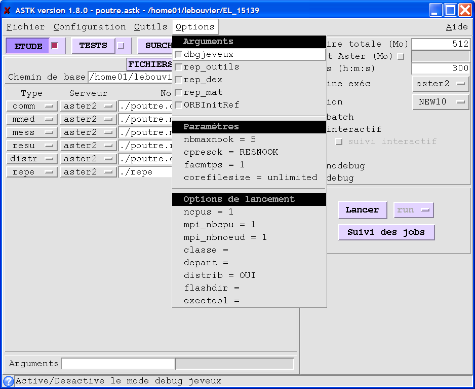
Figure 2.3-b.: distribution option (Astk)
Remarks
Like all Code_Aster calculations, it is possible to launch parametric studies in command line mode with as_run. To do this, it is necessary to have the file.export file in advance:
as_run –serv study_name.export
2.3.1. Management of calculations and results#
The calculation directory is common to that of the results: it is defined in the study profile under the “repe” type. After the execution of the parametric calculations, in this directory there are as many calc_i directories as there are calculations started. There is also a flash directory. Details of each of these directories are presented below.
2.3.1.1. Calculation management#
The command files corresponding to each of the scenarios are automatically generated from the nominal control file and the set of parameters. These files are stored in the calc_i directories.
The output files (message and error) for each calculation are stored in a single directory, the flash directory. All the information concerning the progress of each execution can be found in this directory.
2.3.1.2. Managing results#
As for a classical calculation, the user has the possibility to generate output files (tables, graphs,…). He will have to define them in the standard command file. These outputs will be common to all calculation scenarios.
For example, suppose the user wants to print a table in logical unit file 38 and a result in med format in logical unit file 39. In the nominal command file, he must define the name of each of the output files so that they can be stored in the REPE_OUTproduit directory automatically by*Code_Aster.* The command file extract below illustrates this definition:
DEFI_FICHIER (UNITE =38, FICHIER ='. /REPE_OUT /table.out ')

IMPR_TABLE (TABLE = SIYY, UNITE =38, NOM_PARA =( 'NOEUD', 'SIYY'));


DEFI_FICHIER (UNITE =39, FICHIER ='. /REPE_OUT /beam.rmed ')

IMPR_RESU (FORMAT =' MED ', UNITE =39, RESU =_F (RESULTAT =depl))
Figure 2.3.1.2-a : definition of output files and their logical units
Notes:
In the case of a parametric study the files .messand .resune are not created. However, consulting the files in the.flash directory makes it possible to collect the information usually sent in the* .mess directory.
2.3.1.3. Directory tree#
The figure below shows the location of files and directories for 2 calculation scenarios.
2.4. Additional features#
2.4.1. Generate a base#
As with a standard study, it is possible to generate a database. To do this, simply add a “base” entry to the study profile with the name of the repe directory as the name of the repe directory. For each of the calculation scenarios, the corresponding database stored in the calc_i/base directory will be found.
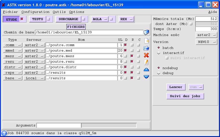
Figure 2.4.1-a: Example of a study profile to generate a base by calculation
2.4.2. Perform a chase#
As with a standard study, it is possible to exploit a base. To do this, simply add a “base” entry to the study profile with the name of the repe directory in which each base to be read is present in the calc_i/base directory.
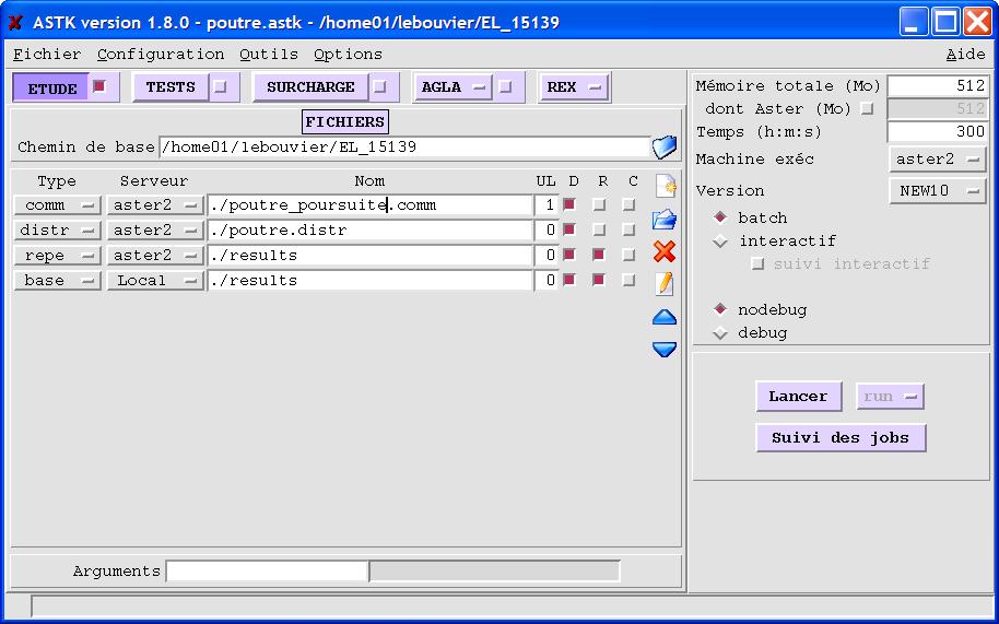
Figure 2.4.2-a: Example of a study profile to exploit the base associated with each calculation
2.4.3. Directory tree#
The directory tree is presented in the presence of a basic reading for each of the 5 calculations. Note the presence of a hostfile, which will be the subject of the next paragraph.
2.4.4. Distribution of calculations#
In the case of parametric studies, the calculations are independent of each other. It is therefore possible to use the available machine resources when distributing calculations. It is therefore necessary to create a “hostfile” defining the machine resources. It defines:
the name of the node where the jobs will be submitted,
the maximum number of jobs to be submitted at the same time,
the total memory allocated.
Note:
On a shared server, it is recommended to use the file defined by the administrator and therefore not to redefine your own resource file.
If the hostfile*file is not present in the study profile, the file* batch_distrib_hostfile*found in the* etc/codeaster*directory will be used by default.*
For example, on the centralized server, resources are managed by the batch software. In this case, the hostfile simply declares the number of calculations that will be submitted at the same time. Here you can submit up to 32 calculations on each front-end node (the memory is indicated*infinite, i.e. you let the batch software manage):
[:ref:`ataster1 <ataster1>`]

cpu=32

mem=9999999


[:ref:`ataster2 <ataster2>`]

cpu=32

mem=9999999
Figure 2.4.4-a : Example file hostfile with batch server
For your resource file to be taken into account, simply add it to your study profile by specifying the type “hostfile”.
In the case of using a set of machines available interactively, the hostfile file could look like:
# node name

[:ref:`machine1 <machine1>`]

# number of CPU available

cpu=4

# total machine memory in MB

mem=4000


# node name

[:ref:`machine2 <machine2>`]

# number of CPU available

cpu=8

# total machine memory in MB

mem=4000
Figure 2.4.4-b : Example file hostfile interactively
We can have up to 12 calculations executed simultaneously depending on the available memory distributed on the two machines. If each calculation requires 2 GB of memory, there will be a maximum of two calculations per machine so as not to exceed the total amount of available memory.
2.4.5. Pre/post-treatments common to all calculations#
There are 4 keywords in the « distr » file: PRE_CALCUL, UNITE_PRE_CALCUL, POST_CALCUL, UNITE_POST_CALCUL.
PRE_CALCUL (resp. POST_CALCUL) defines a text (a set of Aster commands) that will be included just after DEBUT (resp. just before FIN).
UNITE_PRE_CALCUL (resp. UNITE_POST_CALCUL) proposes the same operation except that a logical unit number is provided.
This modification is made for all the « comm » files found in the profile.
This possibility is in particular used by the readjustment command MACR_RECAL to add post-processing to each slave calculation.