3. Methodology presentation#
3.1. General principle#
For a complete overview of dynamic substructuring, the reader is invited to consult the reference document [R4.06.02].
As a preamble, it is necessary to recall that the fact of projecting the substructure on a reduced basis necessarily involves an approximation of the results obtained. The role of the modeler is to choose a fairly rich base in order to be able to understand the dynamic behavior of the substructure. The quality of the results depends on the choice of this projection base.
Here we focus on using interface modes. This consists in condensing the behavior of the structure on the interface degrees of freedom and solving the associated eigenvalue problem. The methodology proposed here differs from the general approach (see U2.07.05) in that the interface modes mentioned here are defined in advance. This is a limitation of the approach: interface modes were defined on the assumption that the methodology would be applied to pipes or at least to structures with shapes similar to that of a pipe.
The principle of the methodology is as follows:
a set of modes with blocked interfaces is calculated for each substructure;
for each interface, we give ourselves a set of well-defined modes, which describe its kinematics. These modes were chosen in advance in order to be able to properly represent the deformations of a section of a pipe filled with fluid.
for each substructure, its response is calculated under the effect of each of the interface modes. These modes complement the modes with blocked interfaces.
The response of the overall structure is then determined using the modes thus constructed for each of the substructures. A mathematical description is provided in section 5.
3.2. Illustration on a simple structure#
To graphically illustrate the process, the following visualizations are proposed which illustrate the case of a right beam of square cross section, embedded on its left and divided into 2 substructures noted SD1 and SD2 ().
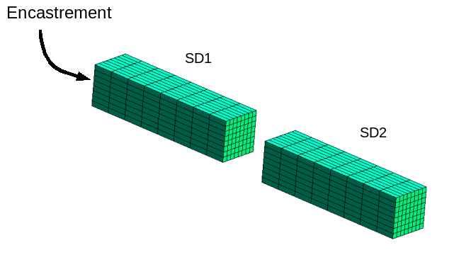
Figure 3.2-1: Beam divided into 2 substructures
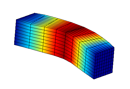
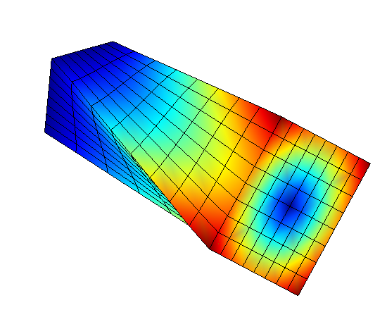
We present the blocked-interface modes of substructure SD1. On the left side applies the embedding related to the modeled problem and on the right side applies the embedding related to the blocking of the interface. This is the first group of modes on which we will reduce the behavior of the SD1 substructure. We do the same on substructure SD2.
|
|
|
|
Mode 1 horizontal |
Mode 1 vertical |
Mode 2 horizontal |
Mode 2 vertical |
Figure 3.2-2: Interface-locked modes
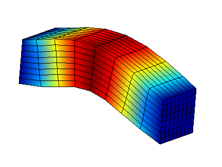
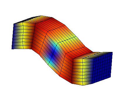
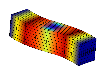
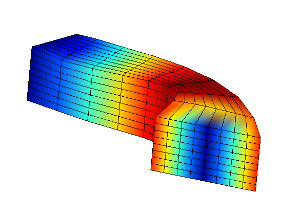
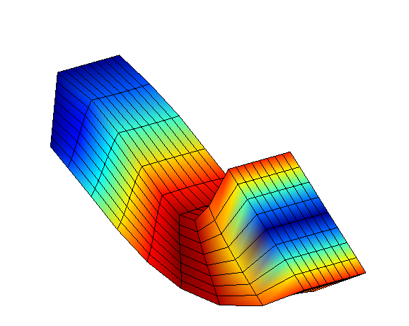
In fact, we present interface modes selected on substructure SD1. These modes have been defined in advance and we can see that they are composed of:
3 unit movements along the X, Y and Z axes [1] _
;
3 unit rotations along the X, Y and Z axes;
1 swelling in the interface plane.
The same construction is carried out on substructure SD2.
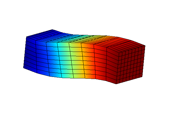
|
|
|
vertical displacement |
horizontal displacement |
axial displacement |
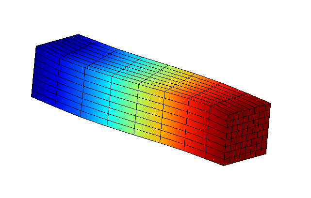
|
|
|
axial rotation |
vertical rotation |
horizontal rotation |
|
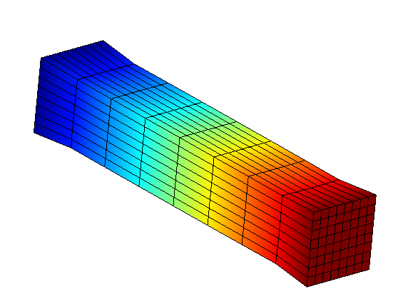
||
swelling |
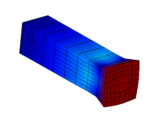
Figure 3.2-3: Effect of interface modes on a substructure
It is then by mixing the local modes and the interface modes of the 2 substructures that we will build the response of the global structure.
It is important to note that the number of interface modes is fixed (in this case by the developer of this methodology) while the number of local modes is at the user’s hand. In the following, we propose recommendations on the number of local modes to remember.
3.3. Extension in case of IFS#
The previous example illustrates the methodology on a purely structural case. The extension to taking into account the interaction with a fluid is natural in this methodology. It essentially involves using the U_P formulation of the problem and defining additional interface modes. Thus, the steps are modified as follows:
local modes become modes with an interface blocked when moving**and* under pressure and they naturally include a structural part and a fluid part;
interface modes consist of structural modes identical to those presented in the previous section to which are added fluid modes: 1 mode with constant pressure on the interface, 2 modes with linear pressure variation respectively along the X axis and along the Y axis of the interface.