4. Practical implementation#
4.1. Prerequisites in terms of modeling and meshing#
We discuss the implementation in code_aster of a modal calculation by dynamic substructuring taking into account IFS. To do this, we define the model problem of a presented lyre. It is a metal pipe through which water flows. The lyre is embedded at each of its ends i.e. the movement of the structure as well as the pressure of the fluid are fixed at 0. The aim is to determine the specific modes of this organ.
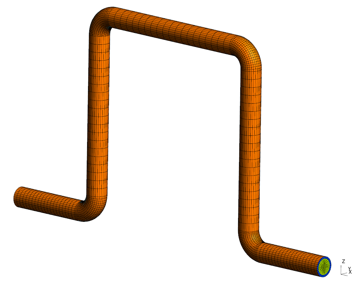
Figure 4.1-1: Model problem of a lyre
On the is presented a section of the lyre: we see in yellow the structural elements and in blue, the fluid elements. The figure shows the components of the degrees of freedom for each of the parts of the model. It can be seen that the nodes shared by the structure and by the fluid carry degrees of freedom of movement and pressure. It should be noted that the mesh must be composed of 3D finite elements and that a fluid-structure modeling U_P must be assigned to it.
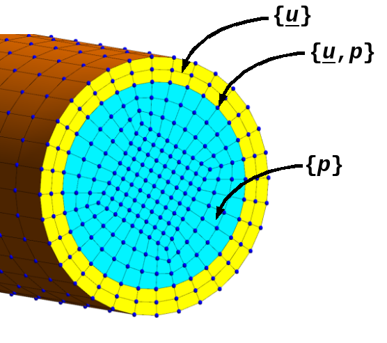
Figure 4.1-2: Lyre section
We are going to use dynamic substructuring to complete this simulation. To do this, you must start by dividing the overall structure into 2 substructures. We therefore need to produce 2 meshes, shown on the. The gap between the 2 substructures is purely artificial in this visualization and is only intended to make the separation into 2 parts visible. For the simulation to be carried out, it is obligatory that an interface surface be created. That is to say that, on the cut between the 2 substructures, a surface must be created and it must have the same name for each one. This is a way to identify interfaces in the case where there are more than 2 substructures.
On the other hand, it is interesting to note that the meshes of 2 interface surfaces do not need to be conforming i.e. their nodes do not need to be coincident.
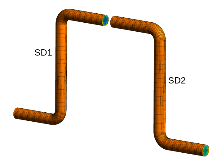
Figure 4.1-3: Divided into 2 substructures
4.2. Conduct of the study#
At the beginning of the command file, import the required objects from the dynamic_substructuring module:
from code_aster.applications.dynamic_substructuring import SubStructure, Structure, Interface |
Once the meshes are read from code_aster and the models are assigned, the resolution steps are as follows. For each substructure: determination of the modes with a blocked interface
Ensure that movement and pressure are blocked at 0 on the interface (AFFE_CHAR_MECA — don’t**not* use AFFE_CHAR_CINE)
Calculation and assembly of mass and stiffness matrices of the substructure (ASSEMBLAGE): for example MASS1, MASS2, RAID1, RAID2
Calculation of modes with a blocked interface (CALC_MODES): for example MODES1, MODES2
Then the definition of the substructures, the interface between them and the calculation of the global response is done as follows, using Python commands:
# definition of substructures subS1 = subStructure (RAID1, MASS1, MODES1) subS2 = subStructure (RAID2, MASS2, MODES2) # definition of the interface according to its name (here “Interface”) interface = Interface (SubS1, SubS2, “Interface”) # calculation of s values of the degrees of freedom at the interface interface.computeInterfaceDofs (“IFS”) # calculation of interface modes Resus_pipe1 = subS1.computeInterfaceModes () Resus_pipe2 = subS2.computeInterfaceModes () # construction of the overall structure myStructure = Structure ([subS1, subS2], [interface]) # calculation of modes global * (here 6) omega, resuSub = mystructure.computeGlobalModes (nmodes=6) |
As an output of the call to the computeGlobalModes method of the MyStructure object, the user gets 2 outputs:
omega: it is a list that contains the natural frequencies of the global structure
ResuSub: this is a list of code_aster result data structures of type MODE_MECA. These are the modes of the global structure projected respectively onto the first and the second substructure (in the order of the global structure definition, here [subS1, subS2]).
4.3. Practical advice#
It is recommended to place the interface between 2 substructures in areas with moderate deformations. In the case of pipes, it is therefore a question of moving away from the elbows, which are the areas where the deformations will be the most important and the least regular.
It is recommended to calculate modes with blocked interfaces up to a minimum frequency of 2 to 3 times the frequency sought on the global structure.
If you want to model 3 substructures SD1, SD2, and SD3 separated respectively by the Int12 and Int23 interfaces as on the, the global structure will be defined as follows:
# construction of the overall structure myStructure = Structure ([SD1, SD2, SD3], [], [Int12, Int23]) |
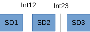
Figure 4.3-1: Case of 3 substructures and 2 interfaces
If you want to model 3 substructures SD1, SD2, and SD3 separated respectively by the interfaces Int12, Int23 and Int31 as on the, the global structure will be defined as follows:
# construction of the overall structure MyStructure = Structure ([SD1, SD2, SD3], [], [Int12, Int12, Int23, Int31]) |
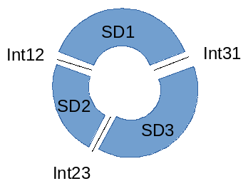
Figure 4.3-2: Case of 3 substructures and 3 interfaces