5. Post-treatments for « rotating machine » studies

For a modal calculation, the*Code_Aster* makes it possible to calculate the modal sensitivities to unbalance as well as the participation coefficients. For harmonic calculations, Code_Aster makes it possible to trace the evolution of the amplitude and the phase of a degree of freedom as a function of the excitation frequency, to trace for a given excitation frequency the deformation of the rotor and the ellipses of the trajectories of the nodes. It also makes it possible to determine the characteristics of the trajectory of the node for a given excitation frequency.

5.1. Modal sensitivities to unbalance

It may happen that a mode (position of its critical speed) is located in an area estimated to be « at risk » without the latter posing any particular vibratory problem. In fact, when the concept of amortization was introduced, the roots of the behavior equation written in matrix form are no longer purely complex, and a real part appears:

\({r}_{i}\mathrm{=}\mathrm{-}\frac{{\epsilon }_{i}{\omega }_{i}}{\sqrt{1\mathrm{-}{\epsilon }_{i}^{2}}}+j{\omega }_{i}\)

Where \({\epsilon }_{i}\) is the reduced damping of the mode and \({\omega }_{i}\) is the natural frequency of the mode. We can then define the unbalance sensitivity factor, \({M}_{i}\):

\({M}_{i}=\frac{{\left(\frac{\Omega }{{\omega }_{i}}\right)}^{2}}{\sqrt{{\left(1-{\left(\frac{\Omega }{{\omega }_{i}}\right)}^{2}\right)}^{2}+4{ϵ}_{i}^{2}{\left(\frac{\Omega }{{\omega }_{i}}\right)}^{2}}}\),

Where \(\Omega\) is the speed of rotation of the shaft line.

This quantity makes it possible to determine whether or not the mode is critical. Thus, a mode that is perfectly synchronous with the speed of rotation may prove to be harmless for the shaft line if its reduced damping has a value close to 1. Therefore, it is considered that if the value of the sensitivity factor is below a certain threshold, then there is no particular vibratory problem. This quantity can be calculated in the following way using concept MODE_MECA:

TABLE = RECU_TABLE (CO= MODES,

NOM_PARA =( “NUME_MODE”, “FREQ”, “AMOR_REDUIT”),);

tab= TABLE. EXTR_TABLE ()

fprop=tab. FREQ

death=tab. AMOR_REDUIT

# Calculation for the nth mode

fp=fprop [i]

am=amort [i]

r=w/fp

N=r**2/sqrt ((1.-r**2) **2.+ (2.*am*r)**2)

5.2. Participation coefficients

For a given mode, the participation coefficients are the respective contributions of the rotor and support deformation energies to the total deformation energy of the system. The total deformation energy of the \(k\) mode is written as:

\({E}_{k}\mathrm{=}{\Phi }_{k}^{t}K{\Phi }_{k}\)

By separating the degrees of freedom relating to the rotor and those relating to the support, energy is expressed in the form:

\({E}_{k}=\left[\begin{array}{c}{\Phi }_{\mathrm{kr}}^{t}{\Phi }_{\mathrm{ks}}^{t}\end{array}\right](\left[\begin{array}{cc}{K}_{r}& 0\\ 0& 0\end{array}\right]+\left[\begin{array}{cc}{K}_{\mathrm{rr}}(\Omega )& {K}_{\mathrm{rs}}(\Omega )\\ {K}_{\mathrm{sr}}(\Omega )& {K}_{\mathrm{ss}}(\Omega )\end{array}\right]+\left[\begin{array}{cc}0& 0\\ 0& {K}_{s}\end{array}\right])\left[\begin{array}{c}{\Phi }_{\mathrm{kr}}\\ {\Phi }_{\mathrm{ks}}\end{array}\right]\)

If we note \({E}_{\mathrm{kr}}\) and \({E}_{\mathrm{ks}}\) the energies of the rotor and the support, defined by:

\({E}_{\mathrm{kr}}={\Phi }_{\mathrm{kr}}^{t}{K}_{r}{\Phi }_{\mathrm{kr}}\) and \({E}_{\mathrm{ks}}={\Phi }_{\mathrm{ks}}^{t}{K}_{s}{\Phi }_{\mathrm{ks}}\)

The participation coefficients relating to the rotor and support are defined respectively by:

\({\rho }_{\mathrm{kr}}=\frac{{E}_{\mathrm{kr}}}{{E}_{k}}\) and \({\rho }_{\mathrm{ks}}=\frac{{E}_{\mathrm{ks}}}{{E}_{k}}\)

The operator POST_ELEM allows direct access to potential, kinetic and elastic deformation energies over the entire mechanical system (option TOUT =” OUI “) or parts of the system (option GROUP_MA =” ROTOR” or GROUP_MA =” MASSIF “). The following example makes it possible to calculate these energies for the first 4 modes of the tree line.

Note:

It is important to note that the calculation of energies is only available for real modes.

EPOT_TOT = POST_ELEM (RESULTAT = MODES,

NUME_MODE =( 1,2,3,4),

MODELE = MODELE,

CARA_ELEM = CARELEM,

CHAM_MATER = CHMAT,

ENER_POT =_F (TOUT =” OUI “),

);

epot_tot= EPOT_TOT. EXTR_TABLE ()

tot_epot=epot_early. TOTALE

EPOT_ROT = POST_ELEM (RESULTAT = MODES,

NUME_MODE =( 1,2,3,4),

MODELE = MODELE,

CARA_ELEM = CARELEM,

CHAM_MATER = CHMAT,

ENER_POT =_F (GROUP_MA =” ROTOR “),

);

epot_rot= EPOT_ROT. EXTR_TABLE ()

rot_epot=epot_rot. TOTALE

EPOT_MAS = POST_ELEM (RESULTAT = MODES,

NUME_MODE =( 1,2,3,4),

MODELE = MODELE,

CARA_ELEM = CARELEM,

CHAM_MATER = CHMAT,

ENER_POT =_F (GROUP_MA =” MASSIF “),

);

epot_mas= EPOT_MAS. EXTR_TABLE ()

mas_epot=epot_mas. TOTALE

Obtaining participation coefficients can be done in Python in the same way as for modal sensitivities to unbalance \({M}_{n}\) (see paragraph 7.1).

# Calculation of rotor and massive participations for the first mode

tot_pot1=tot_epot [1]

rot_pot1=rot_epot [1]

mas_pot1=mas_pot [1]

part_rot=rot_pot1/tot_pot1

part_mas=mas_pot1/tot_pot1

print “part_rot”, part_rot

Print “part_mas”, part_mas

5.3. Determination of phases and amplitudes in harmonics

Deformation (modal, harmonic response, etc.) is characterized by complex displacements. This complex nature of the movements corresponds to the introduction of a phase difference between the movements of the nodes of the model. This phase shift is due to damping and to the gyroscopic effects associated with the rotation of the rotor. From the resulting concept, lateral displacements are recovered in the form of functions as follows:

DY_DIS2 = RECU_FONCTION (RESULTAT = DHAM,

NOM_CHAM =” DEPL “,

NOM_CMP =”DX”,

GROUP_NO =”N_ DIS2 “,);

DZ_DIS2 = RECU_FONCTION (RESULTAT = DHAM,

NOM_CHAM =” DEPL “,

NOM_CMP =”DY”,

GROUP_NO =”N_ DIS2 “,);

The amplitudes and the phases of displacement along the axes \(x\) and \(y\) are obtained from complex modal displacements in the same directions as follows:

MOD_Y_D2 = CALC_FONCTION (EXTRACTION =_F (FONCTION = DX_DIS2,

PARTIE =” MODULE “,),);

MOD_Z_D2 = CALC_FONCTION (EXTRACTION =_F (FONCTION = DY_DIS2,

PARTIE =” MODULE “,),);

PHA_Y_D2 = CALC_FONCTION (EXTRACTION =_F (FONCTION = DX_DIS2,

PARTIE =” PHASE “,),);

PHA_Z_D2 = CALC_FONCTION (EXTRACTION =_F (FONCTION = DY_DIS2,

PARTIE =” PHASE “,),);

For the convenience of implementing subsequent post-processing operations, these quantities are stored in table format.

TABMODY = CREA_TABLE (FONCTION =_F (FONCTION = MOD_X_D2,))

TABMODZ = CREA_TABLE (FONCTION =_F (FONCTION = MOD_Y_D2,))

TABPHAY = CREA_TABLE (FONCTION =_F (FONCTION = PHA_X_D2,))

TABPHAZ = CREA_TABLE (FONCTION =_F (FONCTION = PHA_Y_D2,))

MODYDIS2 = TABMODZ [“DX”,1]

MODZDIS2 = TABMODY [“DY”,1]

PHAYDIS2 = TABPHAZ [“DX”,1]

PHAZDIS2 = TABPHAY [“DY”,1]

5.4. Determination of rotor ellipses

As for the natural modes, the trajectory of a node in the plane perpendicular to the neutral fiber of the rotor is therefore an ellipse whose characteristics are defined in the following way:

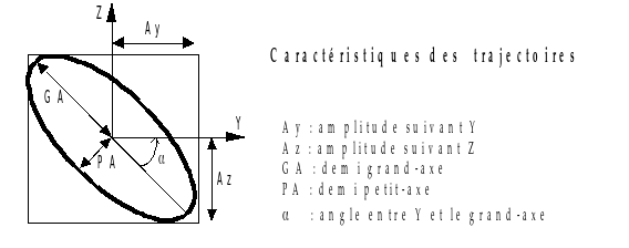
Figure 5.4-a: Illustration of the trajectory of a mode

Next, we need to determine the major axis of the elliptical trajectory. From a vibratory point of view, it is the value of the semi-major axis that represents the vibratory level (peak) to be taken into account for sizing or monitoring.

dax=ellipse (MODXDIS2, MODYDIS2,, PHAXDIS2, PHAYDIS2)

The ellipse function is defined as follows:

def ellipse (modx, mody, thetx, thety):

thetx=thetx*pi/180.

thety=thety*pi/180.

num = modx**2*sin (2*thetx) + mody**2*sin (2*thety)

denum = modx**2*cos (2*thetx) + mody**2*cos (2*thety)

If abs (denum) < 1e-33:

maxhalfaxis = 0.

Else:

T=.5*atan (-num/denum)

ux1 = modx*cos (T+thetx)

uy1 = mody*cos (T+thety)

ux2 = modx*cos (T+Thetx+Pi/2.)

uy2 = mody*cos (T+Thety+Pi/2.)

axy1 = sqrt (ux1**2+uy1**2)

axy2 = sqrt (ux2**2+uy2**2)

maxhalf axis = max (axy1, axy2)

Return maxhalf axis

The direction of travel of the trajectory is called the direction of precession. If the direction of travel of the elliptical trajectory corresponds to the direction of rotation of the rotor, the precession is said to be direct. Otherwise, precession is said to be reverse or retrograde.

It is assumed without proof that, for the same mode, all the nodes have the same sense of precession. We then speak of direct or retrograde mode.

In Code_Aster, the identification of the direction of precession is done either according to the sign of the largest orbit (the node whose major axis is maximum) in a mode, or according to the sign of the sum of the signs of all the orbits. For more information on calculating the sense of precession, the reader can refer to the document [R7.10.03].

5.5. Campbell diagram

The Campbell diagram is a graphical representation that allows the monitoring of the natural frequencies of a rotating system as a function of its rotation speed as well as the zones of instability of these modes ([R7.10.03]). The natural frequencies and the modes of a rotating system are obtained by solving the dynamic equilibrium equation of a system of rotating shafts, without a second member and including the effects of gyroscopic damping.

For this purpose, two macro commands are developed in Code_Aster. The first macro command, CALC_MODE_ROTATION [U4.42.51], allows the calculation of frequencies and modes on the complete system according to rotation speeds. The second macro-command, IMPR_DIAG_CAMPBELL [U4.52.52], makes it possible to classify the flexure, torsional and tensile compression modes, to standardize these modes, to determine the direction of precession of the flexure modes, to sort the frequencies according to various methods of tracking modes and, finally, to draw the Campbell diagram.