2. Numerical modeling of rotating machines#
A study of rotating machines requires both a modeling of the rotating part — the tree line — and a modeling of the support members. It is also possible to take into account the influence of the group table, a structure resulting from civil engineering and on which the support members are based, on the dynamic behavior of the tree line.
2.1. Modeling rotating parts#
Rotors lend themselves quite well to wireframe modeling. From a dynamic point of view, tree lines are flexible elements and it is necessary to take into account transverse shear in the calculation of behavior. This is why a modeling by finite elements of the Timoshenko beam type, taking into account the gyroscopic effect, the shear force deformation and the rotational inertia of the sections, is classically chosen.
However, the theory of beams does not allow sudden changes in section to be treated correctly. In the presence of a significant change in section, the mass involved in the movement corresponds to the geometry of the section. On the other hand, as far as deformation is concerned, it is more limited and the use of the dimensions of the structure to define the sections of the elements results in a strong over-evaluation of the stiffness of the zone in question.
Code_Aster must therefore allow, for each rotor element, a dissociated treatment of the terms of mass and stiffness. Each section of an element is associated with a mass section used to calculate the elementary terms of mass and a stiffness section used to calculate the elementary terms of stiffness. The current data setting of tree line models is therefore done by 2 dual geometries (diameter in stiffness/diameter in mass). This duality mass diameter/stiffness diameter is explained by the \(17°\) rule of thumb. The definition of the mass and the stiffness of each rotor element is based on two different assignments of the elementary characteristics. In general, the mass section corresponds to the geometry of the structure. The stiffness sections may not be consistent with the geometry of the rotor structure, especially in the case of a sudden change in section.
In addition, a three-dimensional modeling of the rotors is also possible in Code_Aster. For more details on the procedure to follow, the reader can refer to the validation documents [V5.03.108], [V5.03.109] and [V5.03.110].
Disks with fins are considered rigid and modelled by equivalent masses and inertias. This makes it possible to neglect the local modes due to the rotor blades and to simplify the structure model. As an example, the schematic representation of a P4-P’4 tree line is visible in the figure below.
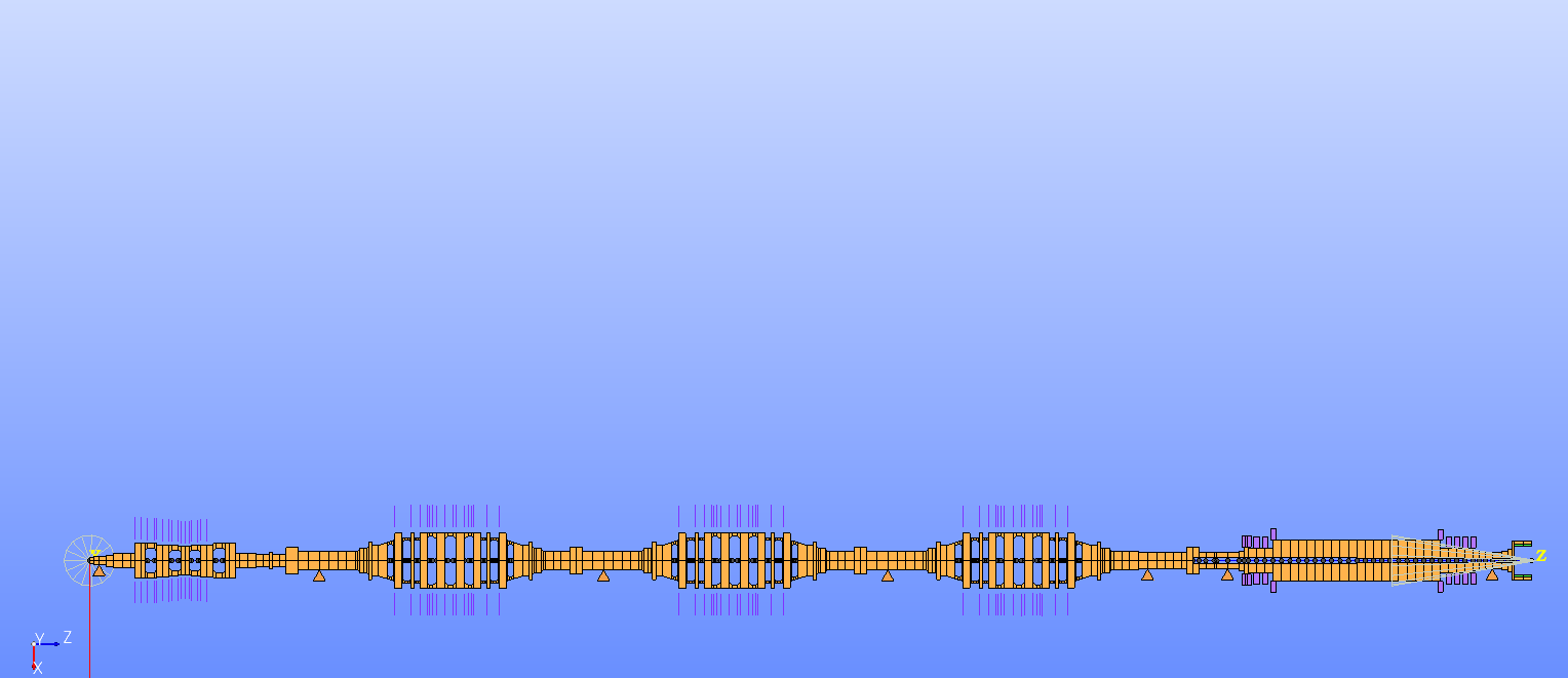
Figure 2.1-a : Representation of a P4-P’4 finite element model
2.2. Modeling of support bearings#
In a turbine in a nuclear power plant, the shaft line is supported by bearings that rest on the mass. This shows the models and notations adopted.
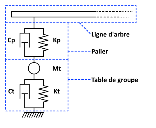
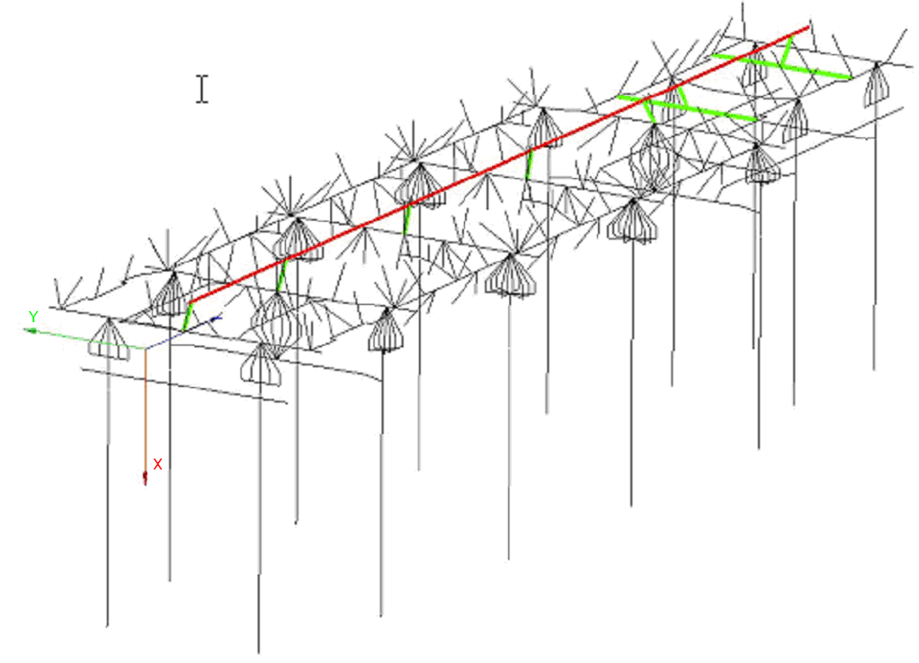
Figure 2.2-a : Representations of the levels and the group table
2.2.1. Linear bearings#
As a first approximation, linear behavior can be retained for the bearings, this behavior being a function of the speed of rotation. In particular, with the hypothesis of small displacements, the stiffness and damping coefficients can be calculated by linearizing the Reynolds equations around the equilibrium position. Then, by calculating the virtual work \({W}_{\mathit{paliers}}\) of the external forces acting on the tree, it comes:
\(\delta {W}_{\mathit{paliers}}\mathrm{=}\left[\begin{array}{c}{F}_{x}{F}_{y}\end{array}\right]\left\{\begin{array}{c}\delta x\\ \delta y\end{array}\right\}\)
with \({F}_{x}\) and \({F}_{y}\) the components of the generalized force acting on the levels.
Assuming that the rotor is perfectly rigid, that the movements of the shaft are limited to the vicinity of a static equilibrium position (index \(0\)) and considering the framework of small disturbances (small displacements \(\left(x,y\right)\) and small speeds \((\dot{x},\dot{y})\)), the components of the forces at the levels are written:
\(\left\{\begin{array}{c}{F}_{x}(x+{x}_{0},y+{y}_{0},\dot{x},\dot{y})\mathrm{=}{F}_{x}({x}_{0},{y}_{0}\mathrm{,0}\mathrm{,0})+x{\left[\frac{\mathrm{\partial }{F}_{x}}{\mathrm{\partial }{x}_{}}\right]}_{0}+y{\left[\frac{\mathrm{\partial }{F}_{x}}{\mathrm{\partial }{y}_{}}\right]}_{0}+\dot{x}{\left[\frac{\mathrm{\partial }{F}_{x}}{\mathrm{\partial }\dot{{x}_{}}}\right]}_{0}+\dot{y}{\left[\frac{\mathrm{\partial }{F}_{x}}{\mathrm{\partial }\dot{{y}_{}}}\right]}_{0}+\text{...}\\ {F}_{y}(x+{x}_{0},y+{y}_{0},\dot{x},\dot{y})\mathrm{=}{F}_{y}({x}_{0},{y}_{0}\mathrm{,0}\mathrm{,0})+x{\left[\frac{\mathrm{\partial }{F}_{y}}{\mathrm{\partial }{x}_{}}\right]}_{0}+y{\left[\frac{\mathrm{\partial }{F}_{y}}{\mathrm{\partial }{y}_{}}\right]}_{0}+\dot{x}{\left[\frac{\mathrm{\partial }{F}_{y}}{\mathrm{\partial }\dot{{x}_{}}}\right]}_{0}+\dot{y}{\left[\frac{\mathrm{\partial }{F}_{y}}{\mathrm{\partial }\dot{{y}_{}}}\right]}_{0}+\text{...}\end{array}\right\}\)
with \({k}_{\mathit{ij}}=-\frac{\partial {F}_{i}}{\partial {x}_{}}\) and \({c}_{\mathit{ij}}=-\frac{\partial {F}_{i}}{\partial \dot{{x}_{j}}}\) which correspond to the stiffness and damping caused by the oil film. These coefficients can be calculated as a function of the geometry of the bearing, which can be found in specialized literature for very simple bearing geometries.
By limiting themselves to the first order, the forces exerted by the fluid on the rotor, following the movements of the center of the rotor, can be put into matrix form:
\(\left\{\begin{array}{c}{F}_{x}\\ {F}_{y}\end{array}\right\}=-\left[\begin{array}{cc}{k}_{\mathit{xx}}& {k}_{\mathit{xy}}\\ {k}_{\mathit{yx}}& {k}_{\mathit{yy}}\end{array}\right]\left\{\begin{array}{c}x\\ y\end{array}\right\}-\left[\begin{array}{cc}{c}_{\mathit{xx}}& {c}_{\mathit{xy}}\\ {c}_{\mathit{yx}}& {c}_{\mathit{yy}}\end{array}\right]\left\{\begin{array}{c}\dot{x}\\ \dot{y}\end{array}\right\}\)
with the terms stiffness and damping matrices described by piecewise linear functions of the speed of rotation. Coefficient values are usually calculated by EDYOS.
2.2.2. Nonlinear bearings#
In general, the nonlinear behavior of bearings can be approximated by a linear representation of the Reynolds equation around an operating point. However, according to REX of studies EDF, for certain fluid levels, where the amplitudes of the vibrations become excessive, it is preferable to take into account non-linear behavior, in particular during the passage of critical speeds where the oil film is strongly crushed.
In the case of turbo-generator sets, the shaft line is supported by hydrodynamic bearings that cannot be considered passive but as elements influencing the dynamic behavior of the shaft line. In fact, the oil film has stiffness and damping properties that vary according to the operating regime of the turbine, i.e. of the eccentricity of the rotor and the speed of rotation (especially at critical speeds), and control the stability of the assembly.
The reactions at the stages are obtained after integration of the pressure field calculated from the non-linear Reynolds equation. The simultaneous resolution of the equations of rotor motion and the hydrodynamic behavior of each bearing can be complex and costly in terms of calculation time.
The consideration of non-linear levels for the calculation of rotating machines is achieved by the coupling between Code_Aster and EDYOS via YACS.
2.3. Group table modeling#
The landings, via the landing chairs, are based on a structure derived from Civil Engineering: the group table. This table, composed mainly of beams and crosspieces, is relatively difficult to model. In the majority of rotating machine studies, we are satisfied with a very simple modeling. Three types of modeling are available:
rigid support
simplified support
widespread support
2.3.1. Rigid support#
In a « rigid support » model, the group table is not modeled and the level (linear or non-linear) is directly connected to an embedded node. The group table is then undeformable and does not allow the transmission of vibrations between the bearings. It is then sufficient simply to impose embedding-type boundary conditions on the nodes connected to the bearings.
2.3.2. Simplified support#
In a « simplified support » model, the group table is modelled by discrete elements characterized by a mass-spring-damper system (see left). All you have to do is identify the dynamic characteristics of the group table, and assign them to the discrete elements. The dynamic stiffness of the group table is then integrated into the modeling, however, this approach does not allow the transmission of vibrations between the levels via the group table.
2.3.3. Generalized support#
In a « generalized support » model, the behavior of the support is defined by a modal base calculated beforehand, for example from a 1D, 3D or hybrid 1D-3D modeling of the group table and its static parts (see right). The generalized massif can be taken into account either by direct calculation or by substructuring such as Craig-Bampton or Mac-Neal (cf. doc [U2.06.04] — Instructions for the construction of reduced models in dynamics). For example, test case SDLV132 [U2.04.132] (cf. appendix) illustrates the implementation of a modal tree-line calculation with its generalized mass, the latter being taken into account by substructuring. The procedure used also makes it possible to take into account technological specificities (condenser linked to external turbine bodies, for example).