1. Equation

1.1. Equations of motion

The objective of this part is to present the essential aspects of a tree line calculation. To do this, we are going to study the simple rotor model of the.

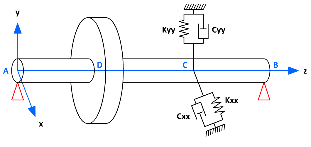
Figure 1.1-a : Simplified Model

The rotor with rotation axis \(z\) is modelled by a beam that has a disk that is one third of its length. On the one hand, it rests on two infinitely rigid supports at each end and, on the other hand, on a linear level in the \(x\) and \(y\) directions located at two thirds of the beam.

Expressions of the kinetic energies of the shaft, disks and bearings are necessary to characterize them. The tree is also characterized by its deformation energy. We also use the forces due to the bearings in order to calculate the virtual work, and thus obtain the corresponding forces exerted on the shaft. Here we will only present the main behavioral equations, without necessarily detailing the calculations to get there.

The general equations of the system are therefore obtained according to the following diagram: for the elements of the system, we calculate the kinetic energy \(T\), the deformation energy \(U\) and the virtual work of the external forces, then we apply the Lagrange equations in the form:

\[\]

: label: EQ-None

frac {d} {text {dt}}}left (frac {partial T} {partial T} {partial {d}}} _ {i}}right) -frac {partial T} {partial T} {partial}} {partial {q}}} {partial T}} {partial T}} {partial T} {partial T} {partial T} {partial T} {partial T} {partial T} {partial}} {partial T} {partial T} {partial}} {partial T} {partial T} {partial}} {partial T} {partial T} {partial T} {partial Q}} {partial T} {partial T} {partial T} {partial Q}}

where \(N\) is the number of degrees of freedom, \({q}_{i}\) are the generalized independent coordinates, and \({F}_{{q}_{i}}\) the generalized forces.

It is assumed that the disk is undeformable, and we are therefore limited to its characterization by its kinetic energy. Thus, the disk is characterized by its inertia matrix at its center of gravity:

\[\]

: label: EQ-None

left [Iright]mathrm {=}left [begin {array} {ccc} {ccc} {I} _ {mathit {xx}} & {mathit {xy}}} & {I}} & {I}} _ {mathit {xz}} _ {mathit {xy}}} & {I} _ {mathit {xy}}} & {I} _ {mathit {xy}}} & {I}} & {I} _ {mathit {xy}}} & {I}}} _ {mathit {yz}}\ {I}} _ {mathit {zx}} _ {mathit {zx}} & {mathit {zy}}} & {I} _ {mathit {zz}}}end {array}right]

The tree is presented as a beam with a constant circular cross section and is characterized by its kinetic and deformation energies.

The terms of stiffness and damping are assumed to be known (see sub-section 2.2.1 for more details on the identification of these coefficients). The forces exerted by the bearing on the shaft can therefore be expressed as:

\[\]

: label: EQ-None

left [begin {array} {c} {F} _ {F} _ {x}\ {F} _ {y}end {array}right]mathrm {-}mathrm {-}left [begin {array} {F} _ {c}} _ {mathit {xx}} _ {mathit {xx}}}\ {K}}{K} _ {mathit {xx}}}\ {K} _ {mathit {xx}} {yx}} & {K} _ {mathit {yy}}}end {array}right]left [begin {array} {c} x\ yend {array}right]mathrm {-}\\ left [begin {array} {yy}}}\ {C}}\ {C} _ {mathit {xy}}\ {C}} _ {mathit {yx}} & {K} _ {mathit {yy}}end {array}right]left [begin {array} {c}dot {x}dot {x}\ dot {x}\ dot {x}\ dot {y}end {array}right]

Figure 1.1-b shows the model and the notations adopted for the bearings while Figure 1.1-a shows a schematic view of the tree line.

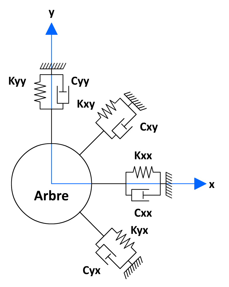
Figure 1.1-b : Linear modeling of the levels

From the calculation of the kinetic energies and deformations of all the elements, and from Lagrange’s equation éq 1.1-1, we obtain behavioral equations that can be rewritten in matrix form (see equation éq 1.1-4):

\(M\text{.}\left[\begin{array}{c}\ddot{x}\\ \ddot{y}\end{array}\right]+C\text{.}\left[\begin{array}{c}\dot{x}\\ \dot{y}\end{array}\right]+\Omega \text{.}G\text{.}\left[\begin{array}{c}\dot{x}\\ \dot{y}\end{array}\right]+K\text{.}\left[\begin{array}{c}x\\ y\end{array}\right]\mathrm{=}\left[\begin{array}{c}{F}_{x}\\ {F}_{y}\end{array}\right]\)

eq 1.1-4

Table 1.1-1

where \(M\), \(C\), \(G\), and \(K\) are, respectively, the square matrices of mass, damping, gyroscopy, and stiffness. We deliberately omit the details of the calculations and refer to the book by Lalanne and Ferraris [1]. It will be noted that the gyroscopy matrix is multiplied by the speed of rotation of the rotor \(\Omega\). The dynamic behavior of the shaft line therefore depends on its speed of rotation. The homogeneous solution of this equation makes it possible to find the frequencies and natural modes of the rotor.