2. Possibilities and limitations of X- FEM in Code_Aster#
This part summarizes the possibilities offered by*Code_Aster* to date, in terms of the use of X- FEM.
Note:
The very first components of X- FEM are available as of version 7, and do not offer much interest. Version 8 corr corresponds to the fruits of the first three years of development, and allows a mechanical calculation in 2D or 3D linear elasticity to be carried out, with 2D or 3D linear elasticity, with boundary conditions far from the crack, itself represented by level sets. Taking into account the contact on the lips of the crack is possible. Version 9 brings many advanced features (multi-cracking, plasticity, etc.). Version 10 offers robust automatic propagation algorithms. In version 11, the X- FEM method is extended to the linear thermal operator in order to take into account the crack initially defined for the mechanical problem in the thermal problem.
2.1. Phenomenon, modeling, and enriched finite elements#
The finite elements X- FEM are only available in mechanic and thermal. It is therefore not possible to model a crack with X- FEM for an acoustic calculation.
For the phenomenon “MECANIQUE “:
The finite elements X- FEM can come from 3D models, C_ PLAN, D_ PLAN or AXIS. On the other hand, the sub-integrated X- FEM elements (*_SI models) are not available.
All geometric mesh types are available:
In 3D:
main meshes: TETRA4, PYRAM5, PENTA6, HEXA8,, TETRA10,, PYRAM13, PENTA15, HEXA20;
edge meshes: TRIA3, QUAD4,, TRIA6, QUAD8.
In Plane Stresses/Plane/Axi-Symmetric Deformations:
main meshes: TRIA3, QUAD4, TRIA6, QUAD8;
edge stitches: SEG2, SEG3.
Attention, quadratic X- FEM elements lack robustness (especially in 3D) and we recommend using linear X- FEM elements.
For the phenomenon “THERMIQUE “:
The finite elements X- FEM can come from 3D models, PLAN, and AXIS.
On the other hand, it is not possible to enrich the other models of this phenomenon: 3D_ DIAG, PLAN_DIAG, AXIS_DIAG, AXIS_FOURIER, COQUE, COQUE_PLAN, COQUE_AXIS.
The following geometric mesh types are available:
In 3D:
main meshes: TETRA4, PYRAM5, PENTA6, HEXA8;
edge stitches: TRIA3, QUAD4
In plane or axisymmetric modeling:
main meshes: TRIA3, QUAD4;
edge stitches: SEG2
Note on the 1D elements of a 3D model:
The 1D edge elements contained in a 3D model cannot be enriched. If these 1D elements are not used in the calculation, it is best not to put them in the model. If they are really used, they should not be close to the crack.
2.2. Law of behavior#
In mechanics, all laws of behavior are available (COMPORTEMENT) in small deformations:
in HPP (small movements and small rotations): DEFORMATION =” PETIT “
in large movements & rotations: DEFORMATION =” GROT_GDEP “.
The other deformation models (for example DEFORMATION =” PETIT_REAC “) are not available.
Note on axi-symmetric modeling:
It is noted that axi-symmetric modeling is only available in small deformation in HPP.
In thermics, the X- FEM method is only available for the operator THER_LINEAIRE: we only treat the case of linear thermics (material parameters independent of temperature). In addition, the thermal conductivity must be isotropic.
2.3. Definition of cracks#
The number of cracks is unlimited. It is also possible to bring them together so that they cut the same element. They can also be connected to each other. The crack bottoms must nevertheless respect a minimum spacing at the neighboring crack: at least two uncut meshes must separate them. This restriction can be circumvented by refining the mesh locally.
Four different ways to define a crack are possible:
or by pre-established geometric shapes (ellipse…) where geometric parameters are requested (semi-major axis…). The pre-established shapes available are the most common cracks: in 2D, crack on a segment or a half-line; in 3D, plane crack with a rectilinear or elliptical bottom, cylindrical crack.**This is the recommended method*.
or by the data of two groups of cells (one for a lip, the other for the bottom of the crack). This method is practical when a crack mesh is already available;
or by the data of the analytical formulas of the level-sets. This method is not suitable for cracks of complex shape;
or by rereading 2 fields to existing nodes.
Thanks to these four methods of defining level-sets, all the scenarios that have been encountered so far have been treated.
An interface is defined in the same way. In fact, only the normal level-set needs to be set.
Notes:
Theoretically, the X- FEM method makes it possible to represent a strong discontinuity (cracks or interface) or a weak discontinuity (interface between glued bi-materials). Everything depends on the enrichment function introduced in the approximation of the displacement or the temperature. In Code_Aster, only a strong discontinuity (field of discontinuous displacements, stresses, or temperatures) is possible [§ 1.1 ] .
2.4. Contact friction#
It is possible to take into account the contact (possibly sliding contact) on the lips of the same crack. The only method allowed is the continuous, wear-free method. It is not possible to define other contact areas. Taking friction into account is not correct in the general case (only very specific configurations work correctly) and it is strongly discouraged to use it. The post-processing of contact degrees of freedom is not easy because the contact table is not completely created if the integration of contact terms is done by the Gauss method.
With the above restrictions, taking into account contact and friction is also possible under the hypothesis of large slides, in 2D as in 3D. This feature is activated as soon as you enter the keyword REAC_GEOM =” AUTOMATIQUE “or REAC_GEOM =” CONTROLE” (key word for the DEFI_CONTACT operator).
The integration scheme used for contact terms is by default a Gauss schema. Other possible patterns are nodal integration, Simpson schemes (3 and 5 points), and Newton-Cotes schemes (4, 5, and 10 points). However, the user is advised to choose integration with nodes.
At present, contact on elements containing the tip of the crack is treated in small and large slides.
In summary, the aspects related to rubbing contact are present on an experimental basis and should not be used for an industrial study.
2.5. Cohesive zones#
It is also possible to take into account the presence of cohesion forces when opening an X- FEM interface. Cohesion is modelled by the cohesive law CZM_EXP_REG already existing in classical finite element method (see [U2.05.07]).
The cohesive law should not be used on elements containing the crack tip in 2D and 3D, but on an interface only.
As with the rubbing contact, the aspects related to cohesive laws are still present on an experimental basis and should not be used for an industrial study.
2.6. Boundary conditions and loads#
Mechanical case
Only certain boundary conditions can be imposed on X- FEM nodes or elements:
DDL_IMPO (DX, DY or DZ) on an X- FEM node (but not on an intersection point),
FACE_IMPO (DNOR or DTAN) on a node X- FEM (but not on a point of intersection),
pressure, force distributed on edge elements X- FEM,
volume force (such as internal force, gravity or rotation) on the elements X- FEM,
pressure on the lips.
In particular, it is not possible to impose a relationship between enriched degrees of freedom, nor to use AFFE_CHAR_CINE on enriched nodes.
To put pressure on the lips of the crack, you cannot use the classic keyword GROUP_MA because no group of elements corresponds to the lips. To do this, you must use AFFE_CHAR_MECA/PRES_REP/FISSURE.
Special case of Dirichlet conditions
There are two ways to impose Dirichlet conditions, the AFFE_CHAR_MECA_R concept and the AFFE_CHAR_MECA_F concept. In the first, the values of the imposed displacements are specified by real values at the nodes of the mesh, while in the second, they are specified throughout the space. In particular, this second concept makes it possible to easily impose discontinuous kinematic conditions through discontinuity.
Active nodes XFEM in the mesh have more degrees of freedom than classic nodes because some fields are enriched.
Concept AFFE_CHAR_MECA_R
When using the AFFE_CHAR_MECA_R concept, for example by submitting a group of nodes whose status is Heaviside to the following condition _F (GROUP_NO =C, DY=α) the code imposes the following linear relationship on each of the nodes in group “A”:
\(\mathit{DY}+\mathit{signe}({\mathit{lsn}}_{\mathit{noeud}})\ast \mathit{H1Y}=\alpha\)
In case of multiple cracks, we will even have the following linear relationship:
\(\mathit{DY}+\Sigma \mathit{signe}({\mathit{lsn}}_{\mathit{noeud},i})\ast \mathit{HiY}=\alpha\)
So for two or more degrees of freedom associated with the DY field, we have a single imposed linear relationship. The boundary conditions are therefore not completely imposed. The DY field will have the desired value at the nodes but nothing is imposed on the DY field at the level of the crack lips. If you simply impose this unique linear relationship on nodes XFEM, unwanted situations may occur, as in the example below:
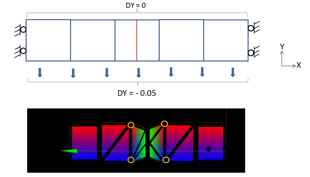
Figure 2.6-a: example of partially imposed Dirichlet conditions
In the example above, the top figure represents the boundary conditions you want to impose. They are imposed using the AFFE_CHAR_MECA_R concept respectively on the top nodes (DY=0) and the bottom nodes (DY=-0.05). Figure shows that the kinematic condition is correctly imposed at the level of nodes XFEM (in orange in the figure) but not at the level of the crack lips. In order to obtain the expected result, namely a uniform stretching of the bar downwards for the lower part of the figure, it is necessary to impose an additional relationship for each XFEM node. The degrees of freedom associated with the DX displacement field will all be fixed in this manner. For example, you can set H1Y=0 to the top nodes and the bottom nodes.
Great care should be taken when the crack lips coincide with a node in the mesh. In this situation, the sign of the normal level-set is undetermined at the node since it is zero. There are then two possibilities when, for example, we impose DY=α using the concept AFFE_CHAR_MECA_R.
First possibility
The kinematic relationship is imposed on either side of the crack (master side and slave side), above and below the interface. The relationship: \(\mathit{DY}=\alpha\) written in the command file then amounts to imposing \(\{\begin{array}{c}\mathit{DY}+\mathit{H1Y}=\alpha \\ \mathit{DY}-\mathit{H1Y}=\alpha \end{array}\) for a node on the interface and therefore blocking any discontinuity of the DY field at this node. ATTENTION, in this case therefore, exceptionally, two relationships instead of one are imposed on the same node. You should not overconstrain this node by also imposing H1Y=0 for example since the matrix will then be non-factorizable. An alarm message to identify the nodes concerned by this configuration is sent. It is important to note that due to the fit to vertex (readjustment of the normal level-set at the node), this situation happens frequently.
Second possibility
The kinematic relationship is only imposed on the master side or only on the slave side, either above or below the interface. The relationship: \(\mathit{DY}=\alpha\) written in the command file is then equivalent to imposing \(\mathit{DY}-\mathit{H1Y}=\alpha\) if it is on the slave side and \(\mathit{DY}+\mathit{H1Y}=\alpha\) if it is on the master side.
The situation where the crack is in accordance with the node is summarized below:
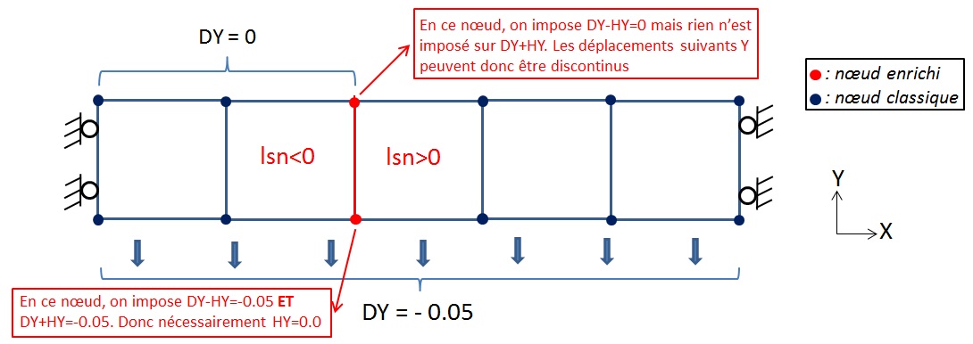
Figure 2.6-b: Crack conforming to the node with concept AFFE_CHAR_MECA_R
Concept AFFE_CHAR_MECA_F
With the AFFE_CHAR_MECA_F concept, Dirichlet conditions are systematically « completely » imposed and it is always possible to impose displacement discontinuities across the crack. To do this, when treating a node belonging to an edge intersected by the discontinuity, we use fictional nodes located on both sides of the crack (in orange in the figure below) to impose the correct values of the classical and enriched degrees of freedom of the node. In fact, the kinematic relationship is evaluated automatically (the user does not need to specify anything) in these fictional nodes to determine the values of the degrees of freedom of the real node XFEM. We thus ensure that the movements are correct both at the nodes and at the level of the crack lips by simply imposing _F (GROUP_NO =C, Dx=f (x, y))
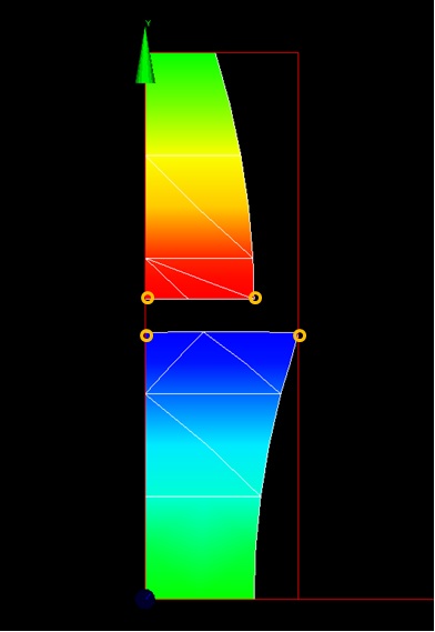
Figure 2.6-c: fictional knots on either side of the crack
When treating an active node XFEM that does not belong to an edge intersected by the discontinuity, you must use other fictional nodes to set the classical and enriched degrees of freedom for this node. The fictional nodes then used are shown in the figures below for linear or quadratic elements, respectively.
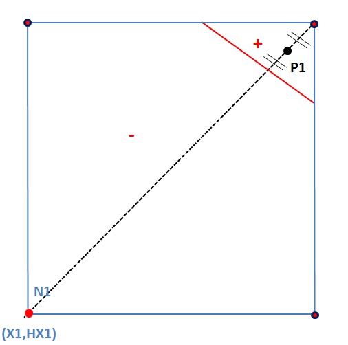
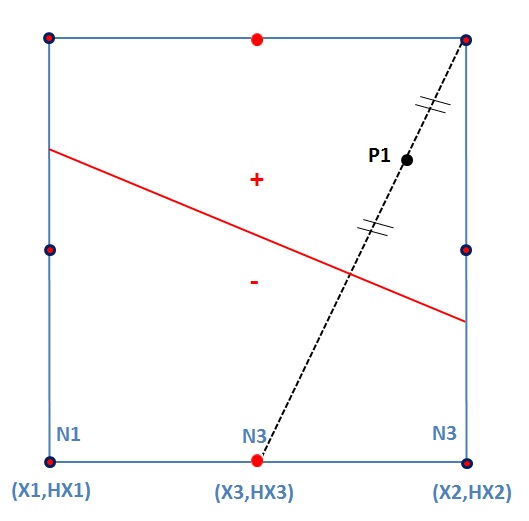
Figure 2.6-d: P1 nodes used for the active nodes XFEM that do not belong to edges intersected by the discontinuity.
Thermal case:
To impose an exchange condition between the lips of the crack, or to impose the continuity of the temperature field across a crack, you must use AFFE_CHAR_THER (or AFFE_CHAR_THER_F)/ECHANGE_PAROI/FISSURE. In the first case we will enter the keyword COEF_H, in the second the keyword TEMP_CONTINUE.
No other boundary conditions can be imposed on X- FEM elements or X- FEM element nodes. Likewise, no source terms can be imposed on X- FEM elements.
The user must therefore make sure to apply his loads sufficiently « far » from the crack, that is to say on non-enriched elements (or nodes belonging to non-enriched elements). It is important to emphasize that as no load is available on the X- FEM edge elements of the thermal models, a zero flow condition is imposed by default on the intersection between the border of the domain in question and the edges of the main X- FEM elements.
2.7. Thermo-mechanical calculation#
There are two possibilities to perform a thermo-mechanical calculation with X- FEM. In both cases, the temperature field is transferred in a conventional manner to mechanical operators (MECA_STATIQUE, STAT_NON_LINE, CALC_G and POST_K1_K2_K3) as a control variable (operator AFFE_MATERIAU, keyword factor AFFE_VARC). These two possibilities differ in the way in which the result of the thermal calculation is produced.
2.7.1. Thermo-mechanical calculation with a healthy thermal model#
The thermal calculation is carried out on a « healthy » thermal model with operators THER_LINEAIRE or THER_NON_LINE. The discontinuity of the temperature field across the crack lips is not modelled. It is therefore a continuous temperature field at the nodes that is transferred to the mechanical operators. This hypothesis constitutes an approximation that should be aware of, but which remains valid for short cracks and/or if we consider an exchange condition between the lips of the crack involving a high value of the exchange coefficient.
Note:
A continuous temperature field at the nodes can also be used as a control variable when a fiel_no*of temperature provided by the user is entered under the simple keyword* CHAM_GD of the factor AFFE_VARC of the operator AFFE_MATERIAU , or when an evol_ther*created on the healthy mesh by the operator* CREA_RESU is entered under the simple keyword EVOL of the operator , or when an evol_ther*created on the healthy mesh by the operator* is entered under the simple keyword of the factor key AFFE_VARC.
2.7.2. Thermo-mechanical calculation with a thermal model X- FEM#
The thermal calculation is carried out on a thermal model X- FEM (functionality only available with the THER_LINEAIRE operator), and the potential discontinuity of the temperature field through the lips of the crack is then taken into account.
Thermo-mechanical chaining with thermal resolution X- FEM and mechanical resolution X- FEM is based on a single mesh, in order to maintain an identical sub-division between thermal and mechanical models. The positions of the integration points are then identical from one model to another, which makes it possible on the one hand to avoid having to project the temperature field, and on the other hand to avoid having to reconstruct the temperature gradient, in particular for the calculation of \(G\) in the CALC_G operator. On the other hand, this choice requires that the displacement field be interpolated by functions of linear form, as is the temperature field.
For this type of chaining, a syntax different from that which is usually used must be adopted in operator MODI_MODELE_XFEM (see [U4.41.11]) when defining the enriched mechanical model (simple keyword MODELE_THER) in order to duplicate the sub-division of the enriched thermal model. The main commands to be used in this case are summarized below.
# definition of crack
FISS = DEFI_FISS_XFEM (MAILLAGE = MA,
DEFI_FISS = _F (…)
# definition of the thermal crack model
MOTH = AFFE_MODELE (MAILLAGE = MA,
AFFE = _F (PHENOMENE = “THERMIQUE”,…))
MOTHX = MODI_MODELE_XFEM (MODELE_IN = MOTH,
FISSURE = FISS)
# resolution on the thermal crack model
THLIX = THER_LINEAIRE (MODELE = MOTHX,…)
# definition of the mechanical model crack
MODELE = AFFE_MODELE (MAILLAGE = MA,
AFFE = _F (PHENOMENE = “MECANIQUE”,…))
MODELX = MODI_MODELE_XFEM (MODELE_IN = MODELE,
MODELE_THER = MOTHX)
# material assignment/control variable
CHAMPMAT = AFFE_MATERIAU (MODELE = MODELX,
AFFE = _F ( … ),
AFFE_VARC = _F (NOM_VARC = “TEMP”,
EVOL = THLIX,…))
# resolution on the mechanical model crack
RESUX = MECA_STATIQUE (MODELE = MODELX,
CHAM_MATER = CHAMPMAT,…)
# mechanical post-treatment of the rupture
TABG = CALC_G (RESULTAT = RESUX,
THETA = _F (FISSURE = FISS,…))
2.8. Hydro-mechanical calculation with an HM- XFEM model#
There is also the possibility of performing a hydromechanical calculation coupled with X- FEM. It is then possible to integrate possibly cohesive hydraulic interfaces into a hydromechanical model, in the same way as with hydraulic joint elements (confer doc [R7.02.15]). The advantage of discretization XFEM is that cohesive interfaces don’t need to be meshed. For more details on how HM- XFEM elements work, refer to the documentation [R7.02.18].
2.8.1. Meshing#
HM- XFEM D_ PLANet 3D elements are available in*Code_Aster*. As for classical HM models, the interpolation of the displacement field is quadratic, these models therefore require exclusively quadratic meshes.
2.8.2. Cohesive interfaces#
In an HM- XFEM model, cohesive interfaces or cracks can be introduced, in the same way as in a classical mechanical model. The types of cohesive zone models available in Code_Aster for HM- XFEM elements are STANDARD (the associated equations are detailed in*2D coupled HM- XFEM modeling with cohesive zone model and applications to fluid-driven fracture network*, M. Faivre, B. network*, M. Faivre, B. PAUL, B., F., F. Golfier, F. Golfier, R. Golfier, R. Giot, P. Giot, P. Massin and D. Colombo, Engineering Fracture Mechanics 2016) and MORTAR (the associated equations are detailed in the documentation [R7.02.12]). With a contact of type MORTAR, we will exclusively use the cohesive law CZM_LIN_MIX, while with a contact of type STANDARD, we will have the choice between the law CZM_OUV_MIX and the law CZM_TAC_MIX.
2.8.3. Material#
Only the « fluid saturated » behavior is available for HM- XFEM models. We therefore define the material in the same way as for conventional saturated HM models, not forgetting to add paragraph RUPT_FRAG if cohesive interfaces have been introduced (in this paragraph we fill in the parameters of the cohesive zone model). In command STAT_NON_LINE, the behavior will also be defined in the same way as for a classic saturated HM modeling: COMPORTEMENT =_F (RELATION = “KIT_HM”, RELATION_KIT =( “ELAS”, “LIQU_SATU”, “”, “HYDR_UTIL”,).
2.8.4. Loads#
With an HM- XFEM model, you can impose the same loads as for a conventional saturated HM model, using the same procedure. But there is an additional loading specific to HM-XFEM models coupled with a cohesive zone model: the imposition of fluid flows directly into the cohesive interfaces. This load is introduced exclusively with the AFFE_CHAR_MECA_F/FLUX_THM_REP command and the FLUN_FISS keyword. It is therefore imposed using a spatial function, on the main elements and not on the edge elements (in fact only the main elements are cohesive). In order to impose such a flow at the level of the mouth of a cohesive hydraulic interface (which is the most widespread case), the function of the non-zero « flow » space is defined at the level of the edge of the domain around the mouth and nowhere else. In the figure on the left, the blue band corresponds to the area where the « flow » space function is defined as non-zero. In this way, the flow is imposed in the mouth (red dot). For 2D models, the mouth of the cohesive interfaces is a point, the imposed flow is therefore punctual and is expressed in kg/s. On the other hand, for 3D models, the mouths are curves (see Figure on the right), the defined flow is therefore a linear flow that is expressed in kg/m/s.
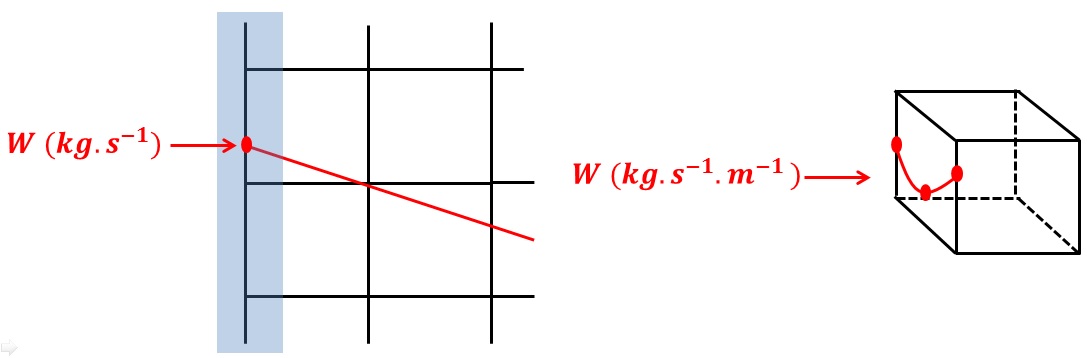
Figure 2.8.4-a: Imposition of a flow at the mouth of a cohesive interface for a 2D model (on the left) and for a 3D model (on the right).
2.8.5. Multi-cracking#
There is the possibility of introducing several interfaces XFEM per element into HM- XFEM models and in particular the possibility of introducing interface junctions, in the same way as in classical mechanics (confer documentation [R7.02.12]: eXtended Finite Element Method)
2.8.6. Base test cases#
The database test cases that concern HM- XFEM models are as follows:
WTNV143: Application of distributed pressure on the lips of a XFEM crack for the hydromechanical case.
WTNV144: Consolidation of a poroelastic and fractured soil column, use of the XFEM method.
WTNV145: Application of distributed pressure on the lips of a XFEM crack junction for the hydromechanical case.
WTNV146: Validation of a cohesive law model for the hydromechanical case coupled with XFEM.
WTNV147: Hydromechanical coupling in a poro-elastic and fractured column, use of the XFEM method.
WTNV148: Flow in an interface within a porous mass: use of the XFEM method.
WTNV149: Contact at the level of a junction of cohesive interfaces for the hydromechanical case.
WTNV150: Flow in an interface junction within a porous mass: use of the XFEM method.
These test cases constitute a panel of examples of how to use the HM- XFEM model. They also validate the functionalities of the model, from the simplest to the most advanced.
2.9. Visualization post-treatments#
Visualizing the results on a healthy network is not very relevant. A specific post-treatment makes it possible to generate a « pseudo- » cracked mesh. This mesh is only intended for post-processing and should not be used for a calculation (it is not a real mesh because it does not respect certain compliance properties in particular).
Then, another post-processing makes it possible to generate, based on the result of the X- FEM calculation and this « pseudo- » cracked mesh:
fields of displacements, constraints and internal variables in mechanics
a thermal temperature field
Then, these fields can be used for other post-treatments (CALC_CHAMP…).
Note:
The passage of a CHAM_ELNOà an CHAM_NOn is not possible because of the « nickname » mesh.
2.10. Mechanics of rupture#
The calculation of the energy return rate \(G\) and the stress intensity factors \({K}_{I}\), \({K}_{\mathit{II}}\) and \({K}_{\mathit{III}}\) is possible either by extrapolation of movement jumps (POST_K1_K2_K3) or by the \(G-\theta\) (CALC_G) method. There are some specific restrictions for X- FEM and CALC_G (see [U4.82.03] for more details).
Note on the calculation of the dynamic stress intensity factor:
It is possible to calculate for X- FEM the dynamic stress intensity factors (for a transitory calculation) and the modal stress intensity factors (associated with modal deformations), see [U4.82.03] for more information.
2.11. Propagation in fatigue#
The PROPA_FISS operator for the automatic propagation of fatigue cracks is available in 2D and 3D.
The PROPA_FISS operator offers 4 methods (METHODE_PROPA = “MAILAGE”, “”, “”, “”, “SIMPLEXE”, “UPWIND”, and “GEOMETRIQUE”), available in 2D and 3D.
As an input, it is necessary to provide him with a table containing the stress intensity factors along the crack base (s) for each crack. These tables should be from CALC_G or POST_K1_K2_K2. Note that all cracks in the structure must be propagated in a single call to operator PROPA_FISS.
The law of propagation is a law of Paris (at each point at the bottom of the crack). The maximum propagation increment at each iteration is imposed by the user.
The angle of bifurcation \(\beta\) and possibly the angle of deviation \(\gamma\) — if the overflow is taken into account — are calculated in PROPA_FISS (the choice of the criterion for calculating the angles of bifurcation is given to the user). The criterion by default is that of the maximum circumferential stress (« maximum hoop stress criterion »). It is also possible to choose previously calculated bifurcation angles. In this case, these angles must have been added in columns BETA and GAMMA of the input table for PROPA_FISS. It should be noted that at present, only method GEOMETRIQUE allows the spill to be taken into account.
Method MAILLAGE (projection) : definition of the 2 level sets based on a mesh of lips and background. In order to propagate the level sets, this mesh is modified at each propagation iteration (METHODE_PROPA =” MAILLAGE “) [11] [12]. Two distinct meshes (crack and structure) are therefore used and only the « mesh » of the crack is modified. Once this « mesh » is updated, the new level sets are recalculated by direct calculation of the distance to the crack (orthogonal projection on the « mesh » of the crack).
Method SIMPLEXE : Resetting the level sets by a fast marching method based on scalar distance calculations. This method is developed for simplex elements (triangles and tetrahedra), but dividing the other meshes into simplexes makes it possible to manage all types of meshes.
Method UPWIND: Resetting the level sets by a fast marching method with discretization to finite differences upwind the reset equation on a regular grid disjoint from the structure. It is presented as an acceleration of the UPWIND method.
Method GEOMETRIQUE: the level sets are recalculated at each propagation step using geometric relationships based on the crack background. This method has no limitations.
Tips on choosing the propagation method are given in § 7.5.
2.12. Various restrictions#
Compatibility with the advanced methods of*Code_Aster* is not assured. In particular, it is impossible to use X- FEM with:
the dynamics,
substructuring,
a model of cohesive zones except those mentioned in § 9.