2. Mechanics#

2.1. Modeling capabilities#

2.1.1. Reminder of formulations#

2.1.1.1. Geometry of plate and shell elements#

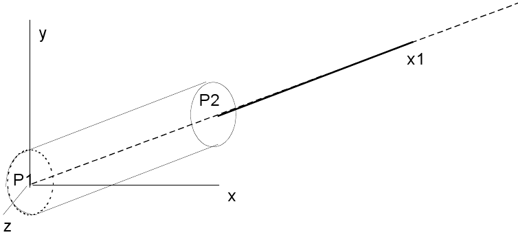
For plate and shell elements, we define a reference surface, or mean surface, which is flat (plane \(\mathit{xy}\) for example) or curved (\(x\) and \(y\) define a set of curvilinear coordinates) and a thickness \(h(x,y)\). This thickness must be small compared to the other dimensions of the structure to be modelled. The figure below illustrates these different configurations.

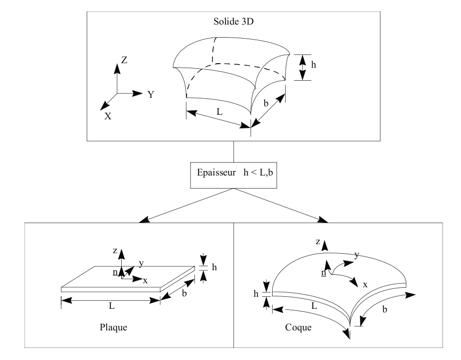
Figure 2.1.1.1-a: Hypothesis in plate and shell theory

A local coordinate system \(\mathit{Oxyz}\) different from the global coordinate system \(\mathit{OXYZ}\) is attached to the mean surface \(\omega\). The position of the points on the plate or shell is given by the curvilinear coordinates \(({\xi }_{\mathrm{1,}}{\xi }_{2})\) of the mean surface and the elevation \({\xi }_{3}\) with respect to this surface. For plates, the curvilinear coordinate system is a local Cartesian coordinate system.

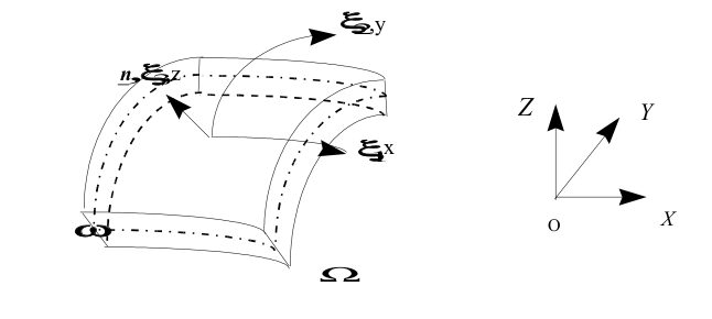
Figure 2.1.1.1-b: Definition of an average area

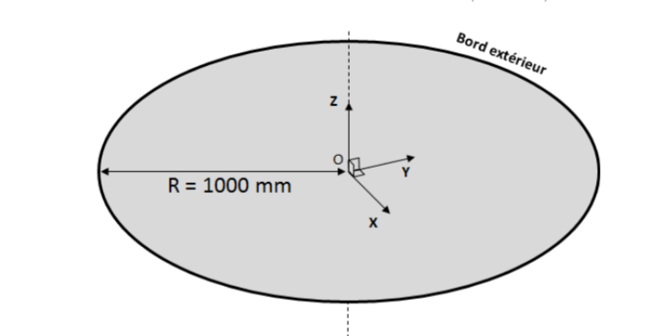
To represent shells with rotational symmetry around an axis (COQUE_AXIS), knowledge of the section of revolution or the trace of the mean surface is sufficient, as shown in figure [Figure 2.1.2.1-a]. These shells are based on a linear mesh and at a point \(m\) of the mean surface a local coordinate system \((n,t,{e}_{z})\) is defined by:

\(t=\frac{{\mathrm{Om}}_{,s}}{∥{\mathrm{Om}}_{,s}∥}\), \(n\mathrm{\wedge }t\mathrm{=}{e}_{z}\)

When you want to model a solid of any shape (not plane), you can use shell elements to account for the curvature, or plate elements. In the latter case, the geometry is approximated by a network of facets.

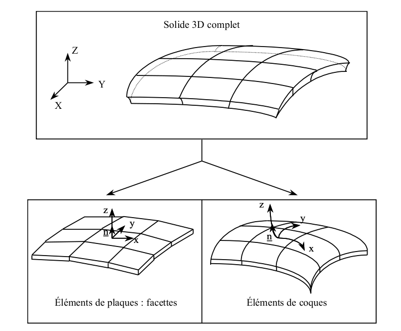
Figure 2.1.1.1-c: Modeling of any 3D solid by plate or shell elements

For the definition of the intrinsic coordinate system, refer to [U4.74.01] paragraph 3.4.

2.1.2. Formulation of plate elements, shells and solid shells#

2.1.2.1. Formulation in geometric linear#

In this formulation, it is assumed that the displacements are small, so we can superimpose the initial geometry and the deformed geometry. These elements are based on shell theory, according to which:

the straight sections that are the sections perpendicular to the reference surface remain straight; the material points located on a normal to the undeformed mean surface remain on a line in the deformed configuration. As a result of this approach,**the displacement fields vary linearly in the thickness of the plate or shell**. If we designate by \(u\), \(v\) and \(w\) the movements from a point \(q(x,y,z)\) to the following \(x\), and, we have: \(y\) \(z\)

\(\left\{\begin{array}{c}u(x,y,z)\\ v(x,y,z)\\ w(x,y,z)\end{array}\right\}=\left\{\begin{array}{c}u(x,y)\\ v(x,y)\\ w(x,y)\end{array}\right\}+z\left\{\begin{array}{c}{\beta }_{x}(x,y)\\ {\beta }_{y}(x,y)\\ 0\end{array}\right\}\)

The associated deformation tensor is then written as: \(\varepsilon (x,y,z)\mathrm{=}e(x,y)+\gamma (x,y)+\mathit{z.}\chi (x,y)\).

The first term \(e\) includes membrane deformations (for a plate element these are the deformations in the plane of the element), the second \(\gamma\) those of transverse shear, and the third \(z\mathrm{.}\chi\) the deflection deformations, associated with the curvature tensor \(\chi\). For thick plates or shells, transverse shears \(\gamma\) are taken into account according to the formulation proposed by Reissner, Hencky, Bollé, Mindlin. This formulation includes the approach without transverse shear, where the tensor \(\gamma\) is zero, developed by Kirchhoff for thin plates or shells according to which the material points located on a normal \(n\) to the mean undeformed surface remain on the normal to the deformed surface.

The transverse stress \({\sigma }_{\mathrm{zz}}\) is zero because it is considered negligible compared to the other components of the stress tensor (hypothesis of plane stresses).
We do not describe the variation in thickness or that of the transverse deformation \({\varepsilon }_{\mathit{zz}}\) which can be calculated using the previous hypothesis of plane stresses.
Taking transverse shear into account depends on correction factors determined a priory by energy equivalences with 3D models, so that the transverse shear stiffness of the plate model is as close as possible to that defined by the theory of three-dimensional elasticity. For homogeneous plates, the transverse shear correction factor based on this method is \(k\mathrm{=}5\mathrm{/}6\).
The shear stresses of the plate elements (DKT /Q, DST /Q, Q/T3G) take into account the possible eccentricity of the elements (free edge hypothesis in particular and quadratic distribution in thickness). However, for two plates that are identical from the material point of view and glued to each other with an eccentricity of their half-thicknesses, the hypothesis of calculating the shear stresses does not make it possible to compare the shear solution with a model composed of a single plate. In fact, in the case of the plate alone, a parabola will be obtained in the thickness cancelling at the ends, in the case of the two plates there will be two parabolas, cancelling at the ends of each plate. To compare two glued plates with a single plate, a use of DEFI_COMPOSITE will be necessary.

Note:

For Mindlin, the determination of correction factors is based on natural frequency equivalences associated with the transverse shear vibration mode. We then obtain \(k\mathrm{=}{\pi }^{2}\mathrm{/}12\) , a value very close to \(5\mathrm{/}6\) .

These elements involve locally:

Five kinematic variables for any plate and shell elements; membrane displacements \(u\) and \(v\) in the reference plane \(z\mathrm{=}0\), transverse displacement \(w\), and rotations \({\beta }_{x}\) and \({\beta }_{y}\) from normal to the mean surface in planes \(\mathit{yz}\) and \(\mathit{xz}\) respectively.
Three kinematic variables for line elements; displacements \(u\) and \(v\) in the reference plane \(z\mathrm{=}0\) and the rotation \({\beta }_{n}\) from normal to the mean surface in plane \(\mathit{xy}\).

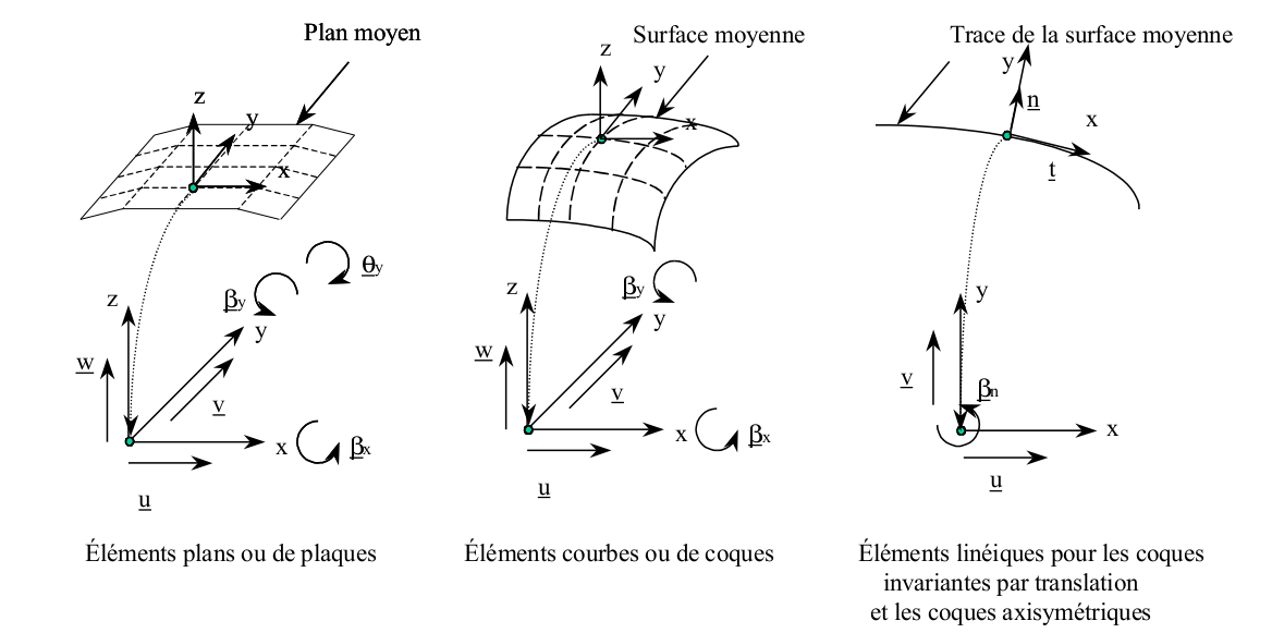
Figure 2.1.2.1-a: Kinematic variables for the various plate and shell elements

Three resulting membrane forces noted \(\mathit{Nxx},\mathit{Nyy},\mathit{Nxy}\) and three moments of bending noted \(\mathit{Mxx},\mathit{Myy},\mathit{Mxy}\) regardless of the plate or shell element; two shear forces noted \(\mathit{Vx}\) and \(\mathit{Vy}\) in the case of any plate and shell elements.

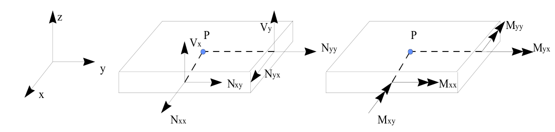
Figure 2.1.2.1-b: Resulting forces for a plate or shell element

2.1.2.2. Formulation in geometric nonlinear, Euler buckling#

In the geometric nonlinear formulation, we are in the presence of large displacements and large rotations, we cannot superimpose the initial geometry and the deformed geometry.

The formulation, described in the reference material [R3.07.05], is based on a 3D continuous medium approach, degenerated by the introduction of Hencky‑Mindlin‑Naghdi shell kinematics into plane stresses in the weak equilibrium formulation. The measurement of the deformations used is that of Green-Lagrange, vigorously combined with Piola-Kirchhoff constraints of the second kind. The equilibrium formulation is therefore a total Lagrangian formulation. Transverse shear is treated in the same way as in the linear case [R3.07.04].

The non-linear element is a volume shell element (COQUE_3D) with a curved mean surface area as presented in the previous paragraph, whose support cells are QUAD9 and TRIA7.

It is possible to apply subsequent pressures to these elements, the formulation of which is described in the reference document [R3.03.07]. This load has the particularity of following the geometry of the structure during its deformation (for example, the hydrostatic pressure always remains perpendicular to the deformed geometry).

Linear buckling also called Euler buckling, described in the reference documentation [R3.07.05] and [R3.07.03], is presented as a particular case of the geometric nonlinear problem. It is based on a linear dependence of the displacement, deformation and stress fields on the load level.

The elements retained in linear buckling are:

the plate element (DKT) with a flat average surface as presented in the previous paragraph, whose support meshes are QUAD4 and TRIA3.
the volume shell element (COQUE_3D) with a curved average surface as presented in the previous paragraph, whose support meshes are QUAD9 and TRIA7.

2.1.3. Comparison between the elements#

2.1.3.1. The differences between plate and shell elements#

The shell elements are curved elements while the plate elements are plane. The variation in the geometry metric (i.e. its radius of curvature) as a function of its thickness is taken into account for shell elements but not for plate elements. This metric variation involves a coupling between membrane and flexure effects for non-planar structures that cannot be observed with planar plate elements for homogeneous material (see [bib1]).

The choice of shape functions for discretizing these elements is different because curved shell elements have a greater number of degrees of freedom. Thus, the plate elements are linear membrane elements while the shell elements are quadratic.

2.1.3.2. The differences between the plate elements#

A distinction is made between elements with transverse shear (DST, DSQ and Q4G) and elements without transverse shear (DKT and DKQ). Elements DST and DKT have triangular support meshes with 3 knots (\(3\mathrm{\times }5\mathrm{=}15\) degrees of freedom) and elements DKQ, DSQ and Q4G have quadrangular support cells with 4 knots (\(4\mathrm{\times }5\mathrm{=}20\) degrees of freedom).

Important note:

For 4-node plate elements (DSQ, * DKQet *Q4G), all 4 nodes must be coplanar for the plate theory to be validated. This check is**systematically performed by Code_Aster, and the user is alarmed if one of the elements of the mesh does not meet this condition. *

In the case of elements with transverse shear, to avoid the blocking of elements under transverse shear (overestimation of stiffness for very small thicknesses), one method consists in constructing constant substitution shear fields at the edges of the element, whose value is the integral of the shear on the edge in question. In Code_Aster, plate and shell elements with transverse shear use this method so as not to block transverse shear. This shear blockage comes from the fact that the elastic shear energy is a term proportional to \(h\) (\(h\) being the thickness of the plate or the shell) much greater than the term of elastic flexural energy which is proportional to \({h}^{3}\). When the thickness becomes small compared to the characteristic length (the \(h/L\) ratio is less than \(1\mathrm{/}20\)), for certain shape functions, the minimization of the predominant term in \(h\) leads to a poor representation of pure flexure modes, for which the deflection is no longer calculated correctly (see [bib1] page 295 with \(h/L=0.01\)).

The Q4G element is a quadrilateral element with four nodes without transverse shear blocking, with bilinear shape functions in \(x\) and \(y\) to represent \(w\), \({\beta }_{x}\), and \({\beta }_{y}\).

The main difference between Q4G modeling and DST comes from the fact that shape functions including a quadratic term are used for the latter to discretize the rotations \({\beta }_{s}\) or \(s\mathrm{=}(x,y)\).

The consequence for the Q4G element is a constant piecewise approximation of the curvatures which involves meshing sufficiently fine in the directions stressed during bending.

Item note DST:

Problems have been highlighted on the triangular element * DST in the case of flexural loading. The results with an equivalent mesh are much worse than those of the DSQ * and depend strongly on the nature of the mesh (see test case ssls141 models E and F V3.03.141). Users are advised to:

to prefer the element DSQà the element DST
on DST to prefer free meshes to regulated meshes (better results)
to avoid asymmetric meshes in relation to the load (if symmetries exist)

2.1.3.3. The differences between shell elements#

Axisymmetric shell elements COQUE_AXIS can be distinguished from elements from COQUE_3D.

The former are used to model \(\mathit{Oy}\) axis revolution structures and the latter in all other cases. For these shell elements, the support meshes are linear at 3 knots. The number of degrees of freedom of these elements is 9.

Any shell elements COQUE_3D have 7-knot triangular or 9-knot quadrangular support meshes:

In the case of triangular cells, the number of degrees of freedom for translations is 6 (the unknowns are the displacements at the vertex nodes and on the midpoints of the sides of the triangle) and that of the rotations is 7 (the unknowns are the 3 rotations at the previous points and at the center of the triangle). So the total number of degrees of freedom of the element is \(\mathit{Nddle}\mathrm{=}3\mathrm{\times }6+3\mathrm{\times }7\mathrm{=}39\).
In the case of quadrangular cells with 9 knots, the number of degrees of freedom for the translations is 8 (the unknowns are the displacements at the vertex nodes and on the midpoints of the sides of the quadrangle) and that of the rotations is 9 (the unknowns are the 3 rotations at the previous points and at the center of the quadrangle). So the total number of degrees of freedom of the element is \(\mathit{Nddle}\mathrm{=}3\mathrm{\times }8+3\mathrm{\times }9\mathrm{=}51\). These elements therefore have about twice as many degrees of freedom as the corresponding plate elements in the DKT family. Their time cost, given the same number, in a calculation will therefore be greater.

The elements in COQUE_3D automatically take into account the metric correction between the average surface and the upper and lower surfaces. For line elements, this correction must be activated by the user (see paragraph 13). Metric correction makes a contribution by \(h/L\) to the constraint and by \({(h/L)}^{2}\) on the go (see [V7.90.03]). For plates, this correction is not applicable.

For shell elements, the shear correction coefficient \(k\) in isotropic behavior can be modified by the user. This shear correction coefficient is given in AFFE_CARA_ELEM under the A_CIS keyword. By default, if the user does not specify anything in AFFE_CARA_ELEM it is equivalent to using the shear theory of REISSNER; the shear coefficient is then set to \(k=5/6\). If the shear coefficient \(k\) is 1 we place ourselves within the framework of the theory of HENCKY - MINDLIN - NAGHDI and if it becomes very large (\(k>{10}^{6.}h/L\)) we approach the theory of LOVE - KIRCHHOFF.

In practice, it is advisable not to change this coefficient. In fact, these elements provide a physically correct solution, whether the shell is thick or thin, with the coefficient \(k=5/6\).

All shell elements found in Code_Aster are protected against shear locking like plate elements (see § 2.1.3.2). Selective integration is used for this [R3.07.03].

However, this property is lost if a displacement field is projected onto a shell element from a calculation on a plate element (with the PROJ_CHAMP command). One should not be surprised at the shear stresses obtained then by a linear calculation based on the displacements (for small thicknesses).

2.2. Commands to use#

2.2.1. Spatial discretization and modeling assignment: operator AFFE_MODELE#

In this part, we describe the choice and assignment of one of the plate or shell models as well as the degrees of freedom and the associated meshes. Most of the information described is extracted from the documentation for using the models ([U3.12.01]: Modeling DKT - DST - Q4G, [U3.12.02]: Modelings COQUE_AXIS).

2.2.1.1. Degrees of freedom#

The degrees of freedom of discretization are in each node of the support mesh the components of displacement at the nodes of the support mesh, unless indicated.

Modeling	Degrees of freedom (at each node)	Remarks
COQUE_3D	DX DY DZ DRX DRY DRZ DRX DRY DRZau central node	The knots belong to the middle leaf of the shell
DKT, DKTG	DX DY DZ DRX DRY DRZ	The nodes belong to the tangent facet at the middle leaf of the shell
DST	DX DY DZ DRX DRY DRZ	The nodes belong to the tangent facet at the middle leaf of the shell
Q4G	DX DY DZ DRX DRY DRZ	The nodes belong to the tangent facet at the middle leaf of the shell
Q 4GG	DX DY DZ DRX DRY DRZ	The nodes belong to the tangent facet at the middle leaf of the shell
COQUE_AXIS	DX DY DRZ	Knots belong to the average surface area of the shell
GRILLE_EXCENTRE	DX DY DZ DRX DRY DRZ	The nodes belong to the facet tangent to the middle leaf of the shell.
GRILLE_MEMBRANE	DX DY DZ	Degree of freedom at all nodes.
MEMBRANE	DX DY DZ	Degree of freedom at all nodes.

2.2.1.2. Stiffness matrix support meshes#

Modeling	Mesh	Finished Element	Remarks
COQUE_3D	TRIA7 QUAD9	MEC3TR7H MEC3QU9H	Meshes not supposed to be flat
DKT, DKTG	TRIA3 QUAD4	MEDKTR3 MEDKQU4	Flat meshes
DST	TRIA3 QUAD4	MEDSTR3 MEDSQU4	Flat meshes
Q4G,	QUAD4	MEQ4QU4	Flat meshes
Q 4GG	QUAD4 TRIA3	MEQ4GG4 MET3GG3	Flat meshes
COQUE_AXIS	SEG3	MECXSE3	Meshes not supposed to be flat
GRILLE_EXCENTRE	TRIA3, QUAD4	MEGCTR3 MEGCQU4	Flat meshes
GRILLE_MEMBRANE	TRIA3, QUAD4, TRIA6, QUAD8	MEGMTR3 MEGMQU4 MEGMTR6 MEGMQU8	Any surface meshes
MEMBRANE	TRIA3, QUAD4, TRIA6,, QUAD8,, TRIA7, QUAD9	MEMBTR3 MEMBQU4 MEMBTR6 MEMBQU8 MEMBTR7 MEMBQU9	Any surface meshes

Modeling GRILLE_EXCENTRE used to model reinforced concrete structures has the same mesh characteristics as modeling DKT

Note:

In a mesh, to transform meshes TRIA6en meshes TRIA7, or QUAD8en meshes QUAD9, you can use the MODI_MAILLAGE operator.

2.2.1.3. Load support meshes#

All the loads applicable to the facets of the elements used here are treated by direct discretization on the support mesh of the element in displacement formulation. Pressure and other surface forces as well as gravity are examples of loads that apply directly to facets. No special loading mesh is therefore necessary for the faces of the plate and shell elements.

For the loads applicable to the edges of the elements, we have:

Modeling	Mesh	Finished Element	Remarks
COQUE_3D	SEG3	MEBOCQ3
DKT, DKTG	SEG2	MEBODKT
DST	SEG2	MEBODST
Q4G	SEG2	MEBOQ4G
Q 4GG	SEG2	MEBOQ4G
COQUE_AXIS	POI1		Support meshes reduced to 1 point
GRILLE_EXCENTRE, GRILLE_MEMBRANE, MEMBRANE			No edge elements affected by these models.

Distributed, linear, tensile, shear forces, and bending moments applied to the edges of shell structures fall into this load category.

2.2.1.4. Model: AFFE_MODELE#

The modeling assignment is done through the operator AFFE_MODELE [U4.41.01].

AFFE_MODELE		Remarks
AFFE
PHENOMENE	“MECANIQUE”
MODELISATION	“COQUE_3D”
	“DKT”
	“DST”
	“DKTG”
	“Q4G”
	“Q 4GG “
	“COQUE_AXIS”
	“GRILLE_MEMBRANE”
	“GRILLE_EXCENTRE”
	“MEMBRANE”

Note:

It is prudent to check the number of items affected.

2.2.2. Basic characteristics: AFFE_CARA_ELEM#

In this part, the operands that are characteristic of plate and shell elements are described. The documentation for using the AFFE_CARA_ELEM operator is [U4.42.01].

AFFE_CARA_ELEM		COQUE_3D	DKT	DKTG	DST	Q4G	Q 4GG	COQUE_AXIS
COQUE
	EPAIS
	/ANGL_REP/VECTEUR
	A_CIS
	COEF_RIGI_DRZ
	EXCENTREMENT
	INER_ROTA
	MODI_METRIQUE
	COQUE_NCOU

AFFE_CARA_ELEM		GRILLE_EXCENTRE	GRILLE_MEMBRANE
GRILLE
	SECTION
	/ANGL_REP/AXE, ORIG_AXE
	EXCENTREMENT
	COEF_RIGI_DRZ

AFFE_CARA_ELEM		MEMBRANE
MEMBRANE
	EPAIS
	/ANGL_REP/AXE, ORIG_AXE
	N_INIT

The characteristics that can be affected on the plate or shell elements are:

The thickness EPAIS is constant on each mesh, since the mesh represents only the middle sheet.
The A_CIS transverse shear correction coefficient for isotropic curved shells.
Taking into account the MODI_METRIQUE metric correction between the average surface and the upper and lower surfaces (effective only for COQUE_AXIS).
A reference direction allowing to define a local coordinate system in the tangential plane at any point in a shell. The construction of the local coordinate system is done either using the two « nautical » angles \(\alpha\) and \(\beta\) (provided in degrees) which define a vector \(v\) whose projection on the tangential plane to the shell fixes the direction \({x}_{l}\). or, if the keyword VECTEUR is present, by the 3 components of the vector \(v\) We can define a single vector \(V\) for the whole structure, or one per zone (keywords GROUP_MA/MAILLE). The construction of the local coordinate system is defined in AFFE_CARA_ELEM [U4.42.01]. This local coordinate system will subsequently be called**user name**.

The definition of this reference axis is also useful for defining the orientation of the fibers of a multilayer or orthotropic shell (see operator DEFI_COMPOSITE [U4.42.03]).

The number of layers COQUE_NCOU used for integration into the thickness of the shell, in operators STAT_NON_LINE and DYNA_NON_LINE (models DKT, COQUE_3D, COQUE_AXIS).
A feature in DEFI_GROUP allows you to automatically create a group of elements whose normal is included in a given solid angle, from axis to reference direction.

This command can be used in pre-processing to assign non-isotropic material data or in post-processing after a shell calculation.

The eccentricity (constant for all the knots in the mesh) EXCENTREMENT of each of them in relation to the support mesh. This distance is measured on the normal of the support mesh. In the eccentric case, rotational inertias are necessarily taken into account and INER_ROTA is set to OUI.
COEF_RIGI_DRZ defines a fictional stiffness coefficient (necessarily small) on the degree of freedom of rotation around the normal to the shell. It is necessary to prevent the stiffness matrix from being singular, but should be chosen as small as possible. For DKT, if we choose COEF_RIGI_DRZ negative, we reinforce by variational writing the kinematics of rotation of the plate element around its normal. We recommend a value of \({10}^{-8}\).

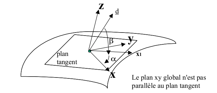
Figure 2.2.2-a: Global coordinate system and tangential plane

For models GRILLE_EXCENTRE and GRILLE_MEMBRANE,

The following geometric data are required to model the reinforcement sheet:

SECTION = \({S}_{1}\): reinforcing bar section in direction 1. The cross section is given per linear meter. It therefore corresponds to the cumulative section over a width of 1 meter. If there is a \(s\) section every \(\mathrm{20.0cm}\), the cumulative section is \(\mathrm{5.s}\).
The orientation of the reinforcements is defined either by
ANGL_REP, to define a vector projected onto the element
or in the case of a cylindrical shell, by ORIG_AXE, AXE to define the angle of the reinforcements, constant in a cylindrical coordinate system.
The eccentricity (constant for all the nodes of the mesh) of the reinforcement sheet in relation to the support mesh (distance measured on the normal of the support mesh), (modeling GRILLE_EXCENTRE only).

To define a grid or if the cross section of the reinforcements in the longitudinal direction and in the transverse direction are different, two layers of elements must be created (crea_mesh command, keyword crea_group_ma), an element layer for the longitudinal direction and a second element layer for the transverse direction:

For linear MEMBRANEen modeling, only the orientation of the membrane’s behavior is necessary. It is defined either by:

ANGL_REP, to define a vector projected onto the element
or in the case of a cylindrical shell, by ORIG_AXE, AXEpour define the angle of the reinforcements, constant in a cylindrical coordinate system.

If we use the non-linear MEMBRANEen we must then fill in:

EPAIS, the thickness of the membrane.
ANGLE_REP, the constraint display frame (only isotropic behavior is possible).
N_INIT, an initial pretension that has the dimension of an effort per unit of length and that disappears after Newton’s increments of the first time step. This pretension is only useful for the convergence of the first time step.

Important note:

The meaning of the normals for each element is a recurring problem concerning the use of this type of element, for example when applying loads of pressure type, or to define an eccentricity or a local coordinate system.

By default for surface elements the orientation is given by the vector product 12^13 for a triangle numbered 123 (DKT,…) or 1234567 (COQUE_3D) and 12^14 for a quadrangle numbered 1234 (DKQ,…) or 123456789 (COQUE_3D). For linear shells \(n\) is given by the formula in paragraph Error: Reference source not found with \(t\) oriented in the direction of travel of the mesh at the mesh level.

Generally, this data can be accessed by looking in the mesh file, which is not very convenient for the user. In addition, he must check the coherence of his mesh and ensure that all the meshes have the same orientation.

The user can automatically change the orientation of mesh elements by imposing a normal direction, for a mesh or part of a mesh using shell models and regardless of the type of modeling. The reorientation of the elements is done using the ORIE_NORM_COQU operator from the MODI_MAILLAGE [U4.12.05] command. The principle is as follows: under ORIE_NORM_COQU, a direction is defined using a vector and a node belonging to the group of elements to be reoriented. If the vector introduced is not in the plane of the mesh selected by MODI_MAILLAGE, a normal direction obtained as the given vector minus its projection on the plane of the mesh is automatically deduced. All the cells in the group related to those initially selected will then have the same normal orientation automatically. Moreover, an automatic verification of the same orientation of the related meshes is carried out using the operator VERI_NORM of the command AFFE_CHAR_MECA [U4.25.01].

2.2.3. Materials: DEFI_MATERIAU#

The behavior of a material is defined using the operator DEFI_MATERIAU [U4.43.01].

Linear MEMBRANE is used with ELAS_MEMBRANE and non-linear with ELAS.

The materials used with all the plate or shell elements can have elastic behaviors under plane stresses whose linear characteristics are constant or functions of temperature.

All nonlinear behaviors under plane constraints (either directly or by the De Borst method [R5.03.03]) are available for DKT and shell models. For more information on these nonlinearities we can refer to paragraph [§ 23].

All nonlinear behaviors in 1D (either directly or by the De Borst method) are available for models GRILLE_EXCENTRE and GRILLE_MEMBRANE.

Thin structures made of composite materials can currently only be treated by plate models, using DEFI_COMPOSITE with homogenized material characteristics. It is also possible to directly introduce the stiffness coefficients of membrane, flexure, and shear matrices with ELAS_COQUE. These coefficients are given in the user coordinate system of the element defined by ANGL_REP. It should be noted that shear terms are only taken into account with behavior ELAS_COQUE for elements DST and Q4G. They are not taken into account with the DKT elements.

In order to facilitate understanding, we have represented the various reference points used in the figure below.

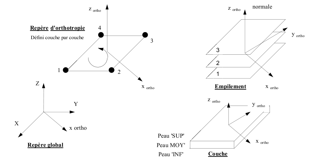
Figure 2.2.3-a: Markers used to define the material

The following example is taken from test case SSLS117B and illustrates the syntax of DEFI_COMPOSITE:

MU2 = DEFI_COMPOSITE (COUCHE =_F (EPAIS =0.2,

MATER = MAT1B,

ORIENTATION =0.0,),);

In this example, we define a multilayer composite of thickness \(0.2\), the material being defined by MAT1B, and the angle of the 1st direction of orthotropy (longitudinal direction or direction of the fibers) being zero. Refer to the [U4.42.03] documentation for more details regarding the use of DEFI_COMPOSITE. (see also [R4.01.01].

2.2.4. Loads and limit conditions: AFFE_CHAR_MECA and AFFE_CHAR_MECA_F#

The assignment of loads and boundary conditions on a mechanical model is performed using the operator AFFE_CHAR_MECA, if the loads and mechanical boundary conditions on a system are real values that do not depend on any parameter, or AFFE_CHAR_MECA_F, if these values are a function of the position or the load increment.

The documentation for using AFFE_CHAR_MECA and AFFE_CHAR_MECA_F is [U4.44.01].

2.2.4.1. List of keywords AFFE_CHAR_MECA factor#

AFFE_CHAR_MECA	COQUE_3D		DKT, DKTG	DST	Q4G,
Q 4GG »	COQUE_AXIS	GRILLE_*
DDL_IMPO
FACE_IMPO
LIAISON_DDL
LIAISON_OBLIQUE
LIAISON_GROUP
CONTACT
LIAISON_UNIF
LIAISON_SOLIDE
LIAISON_ELEM
LIAISON_COQUE
FORCE_NODALE

DDL_IMPO	A factor keyword that can be used to impose one or more displacement values on nodes or groups of nodes.
FACE_IMPO	Keyword factor that can be used to impose, on all the nodes of a face defined by a mesh or a group of elements, one or more displacement values (or of certain associated quantities).
LIAISON_DDL	A factor keyword that can be used to define a linear relationship between degrees of freedom of two or more nodes.
LIAISON_OBLIQUE	A factor keyword that can be used to apply, to nodes or groups of nodes, the same displacement value defined component by component in any oblique coordinate system.
LIAISON_GROUP	Keyword factor that can be used to define linear relationships between certain degrees of freedom of pairs of knots, these pairs of knots being obtained by putting two lists of meshes or knots facing each other.
CONTACT	Keyword factor that can be used to notify contact and friction conditions between two sets of meshes.
LIAISON_UNIF	Keyword factor allowing to impose the same (unknown) value on the degrees of freedom of a set of nodes.
LIAISON_SOLIDE	Keyword factor used to model a non-deformable part of a structure.
LIAISON_ELEM	Keyword factor that makes it possible to model the connections of a shell part with a beam part or a shell part with a pipe part (see paragraph 2.2.4.5).
LIAISON_COQUE	A factor keyword used to represent the connection between shells using linear relationships.
FORCE_NODALE	A factor keyword that can be used to apply, to nodes or groups of nodes, nodal forces, defined component by component in the GLOBALou coordinate system in an oblique coordinate system defined by 3 nautical angles.

AFFE_CHAR_MECA individuals	COQUE_3D	DKT, DKTG	,	DST, Q4G	Q 4GG	COQUE_AXIS	GRILLE_*
FORCE_ARETE
FORCE_COQUE global Near local tangent
PESANTEUR
PRES_REP
ROTATION

PRE_EPSI

FORCE_ARETE	Keyword factor that can be used to apply linear forces to an edge of a shell element. For linear elements, the equivalent is equivalent to applying a nodal force to the element’s support nodes. There is therefore no particular dedicated term. On the other hand, it requires edge elements.
FORCE_COQUE	Keyword factor that can be used to apply surface forces (pressure for example) on elements defined throughout the mesh or on one or more cells or groups of cells. These efforts can be given in the global coordinate system or in a reference frame defined on each cell or group of elements; this coordinate system is built around the normal to the shell element and in a fixed direction (see paragraph 2.2.2).
PESANTEUR	Keyword factor that can be used for heavy-type loading.
PRES_REP	A factor keyword that can be used to apply pressure to one or more meshes, or groups of meshes.
ROTATION	Keyword factor that can be used to calculate the load due to the rotation of the structure.
PRE_EPSI	Keyword factor that can be used to apply an initial deformation loading.

Note:

The pressure forces exerted on the plate elements can be applied either by FORCE_COQUE (near) or PRES_REP. The user should therefore be careful not to apply the pressure load twice for the elements concerned, especially in cases where the plate models would be mixed with other models using PRES_REP.

In addition, it should be noted that the pressure forces, whether with FORCE_COQUE (pres) or PRES_REP, are such that positive pressure acts in the opposite direction to that of normal to the element. By default, this normal depends on the direction in which the nodes of an element travel, which is not always a very easy step for the user.

In addition, this one must ensure that all these elements are oriented in the same way. It is therefore recommended to impose the orientation of these elements using the operator ORIE_NORM_COQU of the MODI_MAILLAGE command (see paragraph [§2.2.2]).

2.2.4.2. List of keywords AFFE_CHAR_MECA_F factor#

The general factor keywords for the AFFE_CHAR_MECA_F operator are the same as those for the AFFE_CHAR_MECA operator shown above.

AFFE_CHAR_MECA_F individuals	COQUE_3D	DKT, DKTG	,	DST	Q4G, Q 4GG	COQUE_AXIS
FORCE_ARETE
FORCE_COQUE global Near local tangent

Pressure loads based on geometry can be entered using FORCE_COQUE (pres).

2.2.4.3. Applying pressure: keyword FORCE_COQUE#

The keyword factor FORCE_COQUE makes it possible to apply surface forces to shell-type elements (DKT, DST, Q4G,…) defined on the entire mesh or on one or more cells or groups of cells. Depending on the name of the operator called, the values are supplied directly (AFFE_CHAR_MECA) or through a function concept (AFFE_CHAR_MECA_F).

	AFFE_CHAR_MECA AFFE_CHAR_MECA_F		Remarks
	FORCE_COQUE:
Global benchmark		TOUT: “OUI” MAILLE GROUP_MA	Place of application of the load
Global benchmark		FX FY FZ MX MY MZ	Supplied directly for AFFE_CHAR_MECA, as a function for AFFE_CHAR_MECA_F
	PLAN	“MOY” “INF” “” SUP “” MAIL “	Allows you to define a force torsor on the average, lower, upper or mesh plane (elements DKTet DST)
Local landmark	PRES	F1 F2 F3 MF1 MF2	Supplied directly for AFFE_CHAR_MECA, as a function for AFFE_CHAR_MECA_F

We refer to the paragraph corresponding to the FORCE_COQUE keyword in the AFFE_CHAR_MECA and AFFE_CHAR_MECA_F operator usage document.

2.2.4.4. Boundary conditions: keywords DDL_IMPOet LIAISON_ *#

The keyword factor DDL_IMPO makes it possible to impose, on nodes introduced by one (at least) of the keywords: TOUT, NOEUD, GROUP_NO, MAILLE, GROUP_MA, one or more displacement values (or of certain associated quantities) to be imposed. Depending on the name of the operator called, the values are supplied directly (AFFE_CHAR_MECA) or through a function concept (AFFE_CHAR_MECA_F).

The operands available for DDL_IMPO are listed below:

DX DY DZ	Blocking on the displacement component in translation
DRX DRY DRZ	Blocking on the rotation displacement component

2.2.4.5. Shell connections with other mechanical elements#

These connections must meet the requirements established in [bib4] and found in particular in the 3D- POUTRE connector in [R3.03.03].

The connections available with the plate and shell elements are as follows:

Beam-Shell Connection: this involves establishing the connection between an end node of a beam element and a group of edge elements of shell elements. Beam and plate theories only know of cuts that are normal to the fiber or to the average surface. Connections can only take place according to these fibers or medium surfaces. The beam-shell connection is **feasible for beams whose neutral fiber is orthogonal to the normal facets of the plates or shells.* Extending it to other configurations (a beam arriving perpendicular to the plane of a plate for example) requires a feasibility study because the plate or shell elements have no stiffness associated with rotation in the plane perpendicular to the normal to the mean surface. The connector can be used using the keyword LIAISON_ELEM: (OPTION: “COQ_POU”) from AFFE_CHAR_MECA.
Shell-Pipe connection: this involves establishing the connection between an end node of a pipe element and a group of edge meshes of shell elements. The formulation of the shell-pipe connection is presented in the reference document [R3.08.06]. The pipe and plate theories only know of cuts that are normal to the fiber or to the average surface. Connections can only take place according to these fibers or medium surfaces. The shell-pipe connection is possible for pipes whose neutral fiber is orthogonal to the normal facets of the plates or shells. The connector can be used using the keyword LIAISON_ELEM: (OPTION: “COQ_TUYAU”) from AFFE_CHAR_MECA.

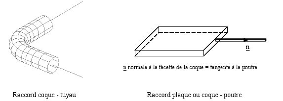
Figure 2.2.4.5-a: Shell connections with other mechanical elements

Shell — 3D massive connection: the massive Shell-3D connection is under study but it will initially be limited to cases where the normal to the solid is orthogonal to the normal to one of the facets of the plate or shell element (see [bib4]).
Connection**between Shell elements**: to connect two shell elements together, we use the AFFE_CHAR_MECA (_F) LIAISON_COQUE keyword (_F) (documentation [U4.44.01]). This connection is made using linear relationships. The classical approach assumes that 2 planes meshed in shells intersect along a line that belongs to the mesh of the structure. In order to prevent the volume that is the intersection of the two shells from being counted twice, the meshing of a shell perpendicular to a given shell is stopped at the level of the upper or lower skin of this last one. On the [Figure 2.2.4.5-b], the connection between the 2 shells is made by solid body connections between the nodes facing each other of the segments \({A}_{1}{A}_{2}\) and \({B}_{1}{B}_{2}\).

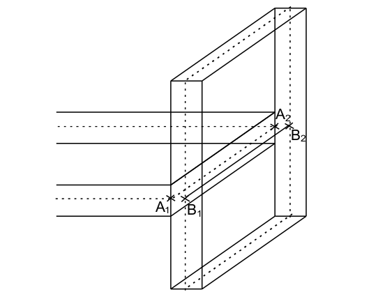
Figure 2.2.4.5-b: Connection between shell elements

Test cases to validate these connections are available in the examples section.

2.2.4.6. Command variables#

The control variables taken into account by the various models are listed here:

Command variables	COQUE_3D	DKT, DST, Q4G	DKTG	Q 4GG	COQUE_AXIS	GRILLE_MEMBRANE GRILLE_EXCENTRE MEMBRANE
TEMP
others: SECH, HYDR, etc.

2.3. Resolution#

2.3.1. Linear calculations: MECA_STATIQUE and other linear operators#

Linear calculations are performed in small deformations. Several linear resolution operators are available:

MECA_STATIQUE:	solving a linear static mechanics problem ([U4.51.01]);

MACRO_ELAS_MULT:	computes linear static responses for different load cases or Fourier modes. ([U4.51.02]).

CALC_MODES:	calculation of eigenvalues and vectors by methods of subspaces or inverse iterations. ([U4.52.02]).

MODE_ITER_CYCL:	calculation of the natural modes of a cyclic symmetric structure ([U4.52.05]);

DYNA_LINE_TRAN:	calculation of the transient dynamic response to any temporal excitation ([U4.53.02]);

DYNA_TRAN_MODAL:	calculation is performed by modal superposition or by substructuring ([U4.53.21]);

2.3.2. Nonlinear calculations: STAT_NON_LINEet DYNA_NON_LINE#

2.3.2.1. Behaviors and deformation hypotheses available#

The following information is taken from the documentation for using the STAT_NON_LINE operator: [U4.51.03].

			COQUE_3D	DKT	DKTG	DST, Q4G	DKTG	Q 4GG	GRILLE_*	COQUE_AXIS
COMPORTEMENT (small deformations)	RELATION	All relationships available in plane constraints
		3D relationships using the De Borst method
		All relationships available in 1D
	DEFORMATION: “GROT_GDEP”	Shell_ 3Den large displacements and large rotations available with nonlinear incremental behaviors, but in small deformations
	DEFORMATION: “PETIT” (or GROT_GDEP)	In small or large displacements available with non-linear incremental behaviors, but with low rotations and small deformations
	DEFORMATION: PETIT or GROT_GDEP	In small or big trips
	RELATION	GLRC_DAMAGE
	RELATION	GLRC_DM, KIT_DDI
COMPORTEMENT (big moves, big rotations)	RELATION	ELAS
	DEFORMATION: “GROT_GDEP”
	TYPE_CHARGE: “SUIV”	Follower pressure

All the mechanical nonlinear behaviors of plane constraints in the code are accessible. The behavioral relationship relates deformation rates to stress rates.

For models GRILLE_EXCENTRE and GRILLE_MEMBRANE, for reinforced concrete structures, 1D nonlinear behaviors correspond to particular incremental behaviors in STAT_NON_LINE (COMPORTEMENT):

GRILLE_ISOT_LINE for isotropic work hardening plasticity,
GRILLE_ISOT_CINE for bi-linear kinematic work hardening plasticity,
GRILLE_PINTO_MEN for Pinto Menegotto’s behavior.

Modeling MEMBRANEest implemented for elastic behaviors in small deformations and small displacements, usable with COMPORTEMENT =” PETIT “and RELATION =” ELAS”, but also for hyper-elastic behaviors in large deformations and large displacements with DEFORMATION =” GROT_GDEP “and RELATION =” ELAS_MEMBRANE_SV “or RELATION =” ELAS_MEMBRANE_NH “.

3D behaviors can also be used using the De Borst method [R5.03.09].

When elements such as plates or shells become coplanar, the stiffness problem should be controlled around the normal range. Indeed, by construction, these elements have no rigidity in this direction: DRZ is a fictitious ddl that avoids the singularity of DKT matrices in global coordinate systems.

The coefficient COEF_RIGI_DRZ in the AFFE_CARA_ELEM operator allows you to modify this value. The default value is sufficient in most cases, but in some situations such as:

thin plate elements used with a large thickness (DKT for example);
a non-linear calculation (STAT_NON_LINE or DYNA_NON_LINE);
DKT elements on twisted quadrangles in general;
COQUE_3D with cinematics of large transformations;
Plate subject to rotation around its normal.

Tip for DKT on COEF_RIGI_DRZ: A bad value penalizes the convergence of calculations. The result, if it is converged, remains just, but the convergence speed is reduced. For example, an elastic linear calculation requires more than one Newton’s iteration to converge. You must then change the value of COEF_RIGI_DRZ and decrease it. However, be careful when choosing this coefficient because a value that is too low can make the matrix singular. It is also possible to enrich the DKT models by taking into account the stiffness according to DRZ. To do this, simply take COEF_RIGI_DRZ negative. In the latter case, we specify that we do not quite have a DKT model as formulated in the literature but we have a DKT model enriched by a kinematics in DRZ: DRZ becomes ddl physical.

Tip for COQUE_3D: In contrast to COQUE_3D, it is better to favor COEF_RIGI_DRZ that is bigger and bigger to avoid singular matrices.

The concept RESULTAT of STAT_NON_LINE/DYNA_NON_LINE contains fields of displacements, constraints, and internal variables at integration points that are always calculated at gauss points:

DEPL: travel fields.
SIEF_ELGA: Constraint tensor per element at integration points (COQUE_3D and DKT) in the user coordinate system. For each layer, we store in the thickness and for each thickness on the surface integration points. So if we want information on a stress for the NC layer, at the level NCN (NCN = -1 if lower, NCN = 0 if middle, NCN = +1 if higher) for the surface integration point NG, we will have to look at the value given by the point defined in the point defined in option POINT such as: NP = 3* (NC-1) NPG + (NCN +1) NPG +NG where NPG is the total number of surface integration points for the element of COQUE_3D (7 for the triangle and 9 for the quadrangle) and the element DKT. For models GRILLE_EXCENTRE, GRILLE_MEMBRANE, we simply store one value per integration point: the component SIXX in the direction of the reinforcements. For models DKTG and Q 4GG, SIEF_ELGA contains the 6 generalized forces (membrane forces, bending moments, shear forces) per Gauss point. In the general case, SIEF_ELGA is a Cauchy constraint field but for COQUE_3D, it is a Piola-Kirchoff constraint field of the second kind.
VARI_ELGA: Field of internal variables (DKT and COQUE_3D) per element at the surface integration points. For each surface integration point, layer information is stored starting with the first layer, level “INF”. The number of variables represented is therefore equal to 2* NCOU * NBVARI where NBVARI represents the number of internal variables.

It can be enriched with the following fields, calculated during post-processing by the operator CALC_CHAMP:

EFGE_ELNO: activates the calculation of the tensor of the generalized forces per element at the nodes (membrane forces, bending moments, shear forces), in the user coordinate system (defined in paragraph [§2.2.2]).
VARI_ELNO: activates the calculation of the internal variables field per element at the nodes in the thickness (by layer SUP/MOY/INF in the thickness unless specified).

2.3.2.2. Details on integration points#

The numbering of the surface Gauss points for elements COQUE_3D is given in R3.07.04 §4.7.1. Pay attention to the order of the Gauss points for the 9-point formula, which is not the same as that adopted for the isoparametric elements.

For models DKT, COQUE_3D, COQUE_AXIS, in the case of non-linear calculations, the integration method for plate and shell elements is an integration method by layers, the number of which is defined by the user. For each layer, except modeling GRILLE, a Simpson method is used with three integration points, in the middle of the layer and in upper and lower layer skins. For \(N\) layers the number of integration points in the thickness is \(\mathrm{2N}+1\).

To treat material nonlinearities, it is recommended to use 3 to 5 layers in the thickness for a number of integration points equal to 7, 9 and 11 respectively. For tangent stiffness, for each layer, under plane stresses, the contribution to the membrane stiffness, and flexure and membrane-flexure coupling matrices is calculated. These contributions are added and assembled to obtain the total tangent stiffness matrix. For each layer, the state of the stresses and all the internal variables are calculated, in the middle of the layer and in the upper and lower layers of the layer. This information is available in VARI_ELGA and SIEF_ELGA. During post-treatment, it is possible to access the values of stress and transverse shear deformation obtained from the derivative of the moments. To do this, an elastic relationship on transverse behavior is even assumed in a non-linear manner.

For models GRILLE_EXCENTRE and GRILLE_MEMBRANE of reinforced concrete structures, there is only one integration point per layer.

2.3.2.3. Geometric nonlinear behavior#

Geometric nonlinear calculations (large displacements and large rotations), available with modeling COQUE_3D, are performed using the STAT_NON_LINE operator, using, under the keyword COMPORTEMENT, DEFORMATION = “GROT_GDEP”.

Geometric nonlinear calculations (large displacements and large rotations), available with modeling MEMBRANE, are performed using the STAT_NON_LINE operator, using, under the keyword COMPORTEMENT, DEFORMATION = “GROT_GDEP”.

Geometric nonlinear calculations (large displacements and small deformations), available with exce modeling, are performed using the STAT_NON_LINE operator, using, under the COMPORTEMENT keyword, DEFORMATION = “GROT_GDEP”.

It is possible to apply subsequent pressures to the elements of COQUE_3D. This load has the particularity of following the geometry of the structure during its deformation (for example: the hydrostatic pressure always remains perpendicular to the deformed geometry). To take this type of load into account, you must specify the following information in operator STAT_NON_LINE:

STAT_NON_LINE (

EXCIT =_F (CHARGE = near

TYPE_CHARGE = “SUIV”)

The geometric non-linear behavior of structures can present instabilities (buckling, snap-through/snap-back…). The determination and the passage of these limit points cannot be obtained by imposing the load, however the loading control options” DDL_IMPO “or” LONG_ARC “of the operator STAT_NON_LINEpermettent to cross these critical points.

The use of the geometric nonlinear element MEMBRANEen can be tricky because of the strong non-linearities and its lack of flexural rigidity. The following points should be noted:

Use of pretension: the use of an initial pretension via N_INITdans the AFFE_CARA_ELEM [U4.42.01] operator is a particularity specific to structural elements without flexural resistance, it is found in code_aster for cable elements. In fact, a membrane subjected to a force perpendicular to its initial surface, as is the case with pressure, will undergo a rigid body movement which causes the calculation to stop. One way to get around this problem is to create an initial stiffness, called « geometric », to allow the convergence of the first increment. It is then normal for the convergence time of this first time step to be quite long, so do not hesitate to allow a high number of Newton iterations (>100) and to play on the value of the initial voltage N_INIT. Pretension is a generalized effort and is written in the form \({N}_{\mathit{init}}={h\sigma }_{0}\) with \(h\) the thickness and \({\sigma }_{0}\) the prestress. It is advisable to start by taking a low prestress value (for example \(1.E-3\)) and then to increase this value by multiplying it by 10 until convergence is obtained. Moreover, we would prefer to take \(h\) and as independent parameters and then enter \({h\sigma }_{0}\) as an argument under the keyword N_INIT. The value \({\sigma }_{0}\) is sometimes difficult to find but it is only useful for the first step of time, so it can be tested quickly.
Initial force and stiffness: the very high non-linearity of the element implies that convergence may be poor when the force applied is too low compared to the stiffness of the material. It is difficult to quantify this ratio but the user should not hesitate to put a lot of force into the first step of time, even if it means activating the division of the time step via the DEFI_LIST_INST command. This is especially true when applying pressure.
Linear search (and contact): one way to significantly improve convergence is to activate linear search (keyword RECH_LINEAIRE in the STAT_NON_LINE [U4.51.03] command). This is sometimes essential for the convergence of calculations, especially during the first steps of time. Unfortunately, linear search is not compatible with contact problems in code_aster, this may lead to having to split the problems into two parts: a first without contact with the linear search and a second with only contact.
Control: if after varying the value of the initial tension and the value of the initial force we are unable to make the calculation converge at the first increment, it is also possible to use the control (keyword PILOTAGEdans STAT_NON_LINE [U4.51.03]). Piloting is also incompatible with contact.

2.3.2.4. Linear buckling#

Linear buckling calculations are similar to the search for natural frequencies and vibration modes. The problem to be solved is expressed in the form:

Find \((\lambda ,X)\mathrm{\in }(\mathrm{ℝ},{\mathrm{ℝ}}^{N})\) such as \(\mathit{AX}\mathrm{=}\lambda \mathit{BX}\)

where	\(A\)	is the stiffness matrix
	\(B\)	is the geometric rigidity matrix (calculated with option RIGI_GEOMde CALC_MATR_ELEM), available for models DKT, DKTG, COQUE_3D
	\(\lambda\)	is the critical load
	\(X\)	is the buckling mode associated with the critical load

The operator CALC_MODES [U4.52.02] is used to determine the critical load and the associated buckling mode.

2.4. Additional calculations and post-treatments#

2.4.1. Elementary matrix calculations: operator CALC_MATR_ELEM#

The operator CALC_MATR_ELEM (documentation [U4.61.01]) makes it possible to calculate elementary matrices, which can then be assembled by the command ASSE_MATRICE (documentation [U4.61.22]).

The basic options for the CALC_MATR_ELEM operator are described below:

CALC_MATR_ELEM	COQUE_3D	DKT, DKTG	DST	Q4G, Q 4GG	COQUE_AXIS	GRILLE_*
“AMOR_MECA”
“MASS_MECA”
“MASS_INER”
“RIGI_GEOM”
“RIGI_MECA”
“RIGI_MECA_HYST”

AMOR_MECA: Damping matrix for elements calculated by linear combination of stiffness and mass.
MASS_MECA: Mass matrix.
MASS_INER: calculation of inertial characteristics (mass, center of gravity)
RIGI_GEOM: Geometric rigidity matrix (for large movements).
RIGI_MECA: Element stiffness matrix.
RIGI_MECA_HYST: Hysteretic stiffness (complex) calculated by the product by a complex structural damping coefficient of simple stiffness.

2.4.2. Element-based calculations: operators CALC_CHAMP and POST_CHAMP#

Post-treatment options for plate and shell elements are presented below. They correspond to the results that a user can obtain after a thermomechanical calculation (stresses, displacements, deformations, internal variables, etc…). For structures modelled by shell or beam elements, it is particularly important to know how stress results are presented so that they can be interpreted correctly. The approach adopted in Code_Aster consists in calculating the constraints in the « user » coordinate system defined in the AFFE_CARA_ELEM operator.

If you want to extract your results in a coordinate system other than the user coordinate system, you must use the MODI_REPERE command.

When post-processing only concerns a « sub-point », the user has the keywords NUME_COUCHE and NIVE_COUCHE of the factor keyword EXTR_COQUE of the command POST_CHAMP.

The keywords under EXTR_COQUE are described in the following table:

OPTIONS	COQUE_3D	DKT	DST, Q4G	DKTG, Q 4GG	COQUE_AXIS	GRILLE_*
NUME_COUCHE
NIVE_COUCHE

More precisely, in the case of a multilayer material (multilayer shell defined by DEFI_COMPOSITE), or of a structural element with local non-linear behavior, integrated by layers, NUME_COUCHE is the integer value between 1 and the number of layers, necessary to specify the layer where it is desired to perform the elementary calculation. By convention, layer 1 is the bottom layer (in the normal sense) in the case of shell elements.
For the nume layer defined by NUME_COUCHE, allows you to specify the ordinate where you want to perform the elementary calculation: INF/MOY/SUP corresponding to the integration points located in the inner/middle/outer skin of the layer.

The keyword factor COQU_EXCENT makes it possible to modify the generalized forces calculation plan (options EFGE_ELNO and EFGE_ELGA) for a model with plate elements (DKT, DST, Q4G, DKTG) taking into account the eccentricity (MODI_PLAN =” OUI “).

The post-processing options available are:

OPTIONS	COQUE_3D	DKT	DST, Q4G	DKTG, Q 4GG	COQUE_AXIS	GRILLE_*
“ENEL_ELGA” “ENEL_ELNO” “ENEL_ELEM”
“ENER_ELAS”
“EPSI_ELGA”
“SIEQ_ELGA”
“DEGE_ELGA”
“DEGE_ELNO”
“ECIN_ELEM”
“EFGE_ELGA”
“EFGE_ELNO”
“EPOT_ELEM”
“EPSI_ELNO”
“SIEQ_ELNO”
“SIEF_ELGA”
“SIEF_ELNO”
“SIGM_ELNO”
“VARI_ELNO”

SIEF_ELGA: Calculation of the generalized efforts per element at the points of integration of the element based on the movements (use only in elasticity). User coordinate system.
SIGM_ELNO: Calculation of the constraints per element at the nodes. User coordinate system. These are the Cauchy constraints.
SIEQ_ELNO: Constraints equivalent to nodes, calculated at one point in the thickness from SIGM_ELNO:

VMIS: Von Mises constraints.

VMIS_SG: Von Mises constraints signed by the constraint trace.

PRIN_1, PRIN_2, PRIN_3: Main constraints.

These constraints are independent of the frame of reference.

EFGE_ELGA: Calculation of the generalized efforts per element at the points of integration of the element based on the movements (use only in elasticity). User coordinate system.
EFGE_ELNO: Calculation of the generalized forces per element at the nodes based on the displacements (use only in elasticity). User coordinate system.
EPSI_ELNO: Calculation of the deformations per element at the nodes from the displacements, at one point in the thickness (use only in elasticity). User coordinate system.
EPSI_ELGA: Calculation of the deformations per element at the integration points based on the displacements, at one point in the thickness (use only in elasticity). Intrinsic coordinate system.
DEGE_ELGA: Calculation of the generalized deformations per element at the points of integration of the element based on the displacements. User coordinate system.
DEGE_ELNO: Calculation of generalized deformations by element at the nodes based on the displacements. User coordinate system.
EPOT_ELEM: Calculation of the linear elastic deformation energy per element from the displacements.
ENER_TOTALE: calculation of the total deformation energy integrated on the element
ENER_ELAS: calculation of the elastic deformation energy integrated on the element
ENEL_ELGA/ENEL_ELNO: elastic energy at integration points or at nodes
ENEL_ELEM: elastic energy on the element
ECIN_ELEM: Calculating kinetic energy per element.
EFGE_ELNO: Option to activate the calculation of the generalized force tensor (see paragraph [§ Calculs non linéaires: STAT_NON_LINE et DYNA_NON_LINE]) per element at the nodes, in the user frame of reference, by integrating the constraints SIEF_ELGA (in non-linear).
EFGE_ELGA: Option to activate the calculation of the generalized force tensor (see paragraph [§ Calculs non linéaires: STAT_NON_LINE et DYNA_NON_LINE]) per element at the gauss points of the element, in the user coordinate system, by integrating the constraints SIEF_ELGA (non-linear).
VARI_ELNO: Option to activate the calculation of the internal variables field by element and by layer at the nodes. For each surface integration point, layer information is stored starting with the first layer, level “INF”. The number of variables represented is therefore equal to 3* NCOU * NBVARI where NBVARI represents the number of internal variables.
NUME_COUCHE: In the case of a multilayer material (composite or plastic shell), integer value between 1 and the number of layers, necessary to specify the layer where you want to perform the elementary calculation.
NIVE_COUCHE: For layer \(n\), you can specify the ordinate where you want to perform the elementary calculation. A calculation in the inner skin is indicated by “INF”, in the outer skin by “SUP” and on the middle sheet by “MOY” (depending on the normal direction).

2.4.3. Node calculations: operator CALC_CHAMP#

OPTIONS	COQUE_3D	DKT	DST	Q4G	COQUE_AXIS	GRILLE
“FORC_NODA”
“REAC_NODA”
_ NOEU

For plate and shell elements, the operator CALC_CHAMP (documentation [U4.81.04]) only allows the calculation of forces and reactions (calculation of the fields at the nodes by averaging, option _ NOEU):

based on the constraints, the balance: FORC_NODA (calculation of nodal forces based on the constraints at the integration points, element by element),
then by removing the load applied: REAC_NODA (calculation of the nodal forces of reaction to the nodes, based on the constraints at the integration points, element by element):
REAC_NODA = FORC_NODA - loads applied,
useful for load verification and for calculating results, moments, etc.

2.4.4. Quantity calculations on all or part of the structure: operator POST_ELEM#

The operator POST_ELEM (documentation [U4.81.22]) allows quantities to be calculated on all or part of the structure. The quantities calculated correspond to particular calculation options of the affected modeling.

MASS_INER: calculation of geometric characteristics (volume, center of gravity, inertia matrix) for plate and curved elements.
ENER_POT: calculation of the potential deformation energy at equilibrium from the displacements in linear mechanics of continuous media (2D and 3D) and in linear mechanics for structural elements, or the energy dissipated thermally at equilibrium in linear thermal equilibrium from temperatures (cham_no_ TEMP_R).
ENER_CIN: calculation of kinetic energy from a speed field or from a displacement field and a frequency (only for structural elements and 3D elements).
ENER_ELAS: calculation of the elastic deformation energy.

2.4.5. Quantity field component values: operator POST_RELEVE_T#

The operator POST_RELEVE_T (documentation [U4.81.21]) allows, on a group of nodes, to extract values or perform calculations:

to extract values from components of quantity fields;
to perform calculations of averages and invariants:
Average,
Results and moments of vector fields,
Tensory field invariants,
Directional trace of fields,
Expressed in the references GLOBAL, LOCAL,, POLAIRE,, UTILISATEUR, or CYLINDRIQUE

The product concept is a table type.

To use POST_RELEVE_T, you need to define three concepts:

a**location**: the NODE option (example: N01 N045) or the option GROUP_NO (example: APPUI);
a**object**: either option RESULTAT (SD result: EVOL_ELAS,…) or option CHAM_GD (CHAM_NO: DEPL,… or CHAM_ELEM: SIGM_ELNO,…);
a**natural**: either the option “EXTRACTION” (value,…) or the option “MOYENNE” (average, max, mini,…).

Important note:

If you come from an interface with a mesher, the knots are arranged in numerical order. The nodes must be reordered along the stripping line. The solution is to use the operator DEFI_GROUP with the option NOEU_ORDO. This option allows you to create a GROUP_NOordonné containing the nodes of a set of meshes made up of segments (SEG2ou * SEG3) .

An example of component extraction is given in test case SSNL503 (see description in paragraph [§2.5.3] page 36):

TAB_DRZ = POST_RELEVE_T (ACTION =_F (

GROUP_NO = “D”,

INTITULE = “TB_DRZ”,

RESULTAT = RESUL,

NOM_CHAM = “DEPL”,

NOM_CMP = “DRZ”,

TOUT_ORDRE = “OUI”,

OPERATION = “EXTRACTION”

The purpose of this syntax is:

to extract:	OPERATION = “EXTRACTION”
on the group of nodes \(D\):	GROUP_NO = “D”
the \(\mathit{DRZ}\) component of the move:	NOM_CHAM = “DEPL”, NOM_CMP = “DRZ”,
for all calculation times:	TOUT_ORDRE = “OUI”

2.4.6. Printing results: operator IMPR_RESU#

The IMPR_RESU operator allows you to write the mesh and/or the results of a calculation on listing in the format “RESULTAT” or on a file in a format viewable by post-processing tools external to Aster: format RESULTAT and ASTER (documentation [U4.91.01]), format CASTEM (documentation []), format (documentation []), format IDEAS (U7.05.11 documentation [U7.05.01]), MED format (documentation [U7.05.21]), or format GMSH (documentation [U7.05.32]).

This procedure allows you to write as you wish:

a mesh,
from fields to nodes (movements, temperatures, natural modes, static modes,…),
fields by elements at the nodes or at the points of GAUSS (constraints, generalized efforts, internal variables…).

Since plate and shell elements are treated in the same way as other finite elements, we refer the reader to the usage notes corresponding to the output format they want to use.

2.5. Examples#

The test cases selected here are classic test cases from the literature and which are commonly used to validate this type of element.

We recall that the DKT models correspond to the Love-Kirchhoff theory and the DST, Q4G models correspond to the theory with transverse shear energy (Reissner). The results for modeling COQUE_3D are only presented for a theory with transverse shear energy.

2.5.1. Linear static analysis#

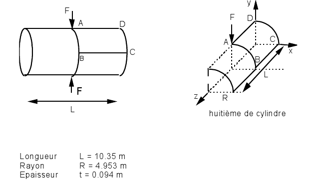
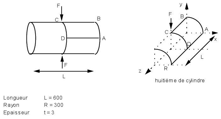
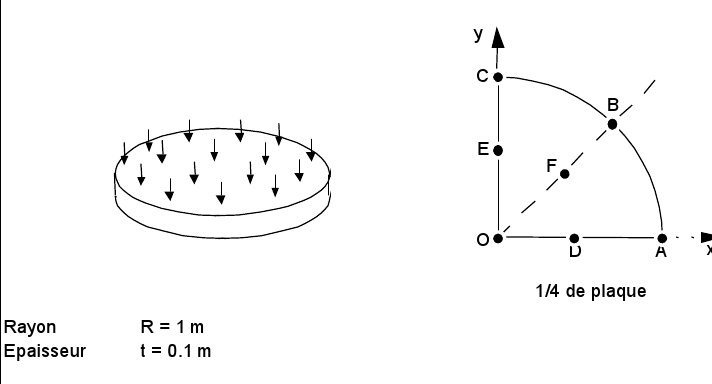
SSLS20	Title:: Pinched cylindrical shell with free edges Documentation V: [] Modelings: SSLS20A DKT SSLS20B COQUE_3D MEC3QU9H SSLS20C COQUE_3D MEC3TR7H

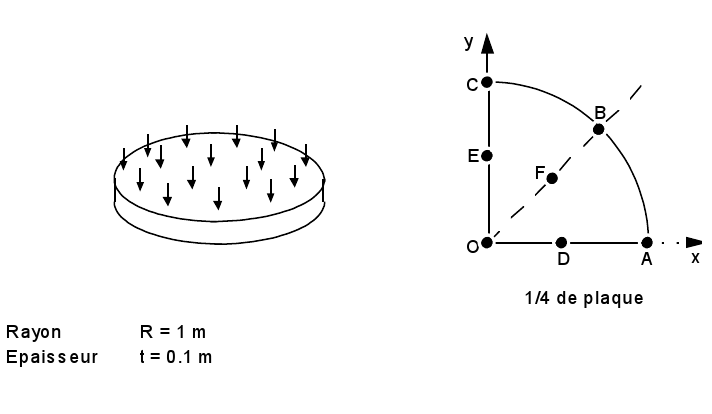
SSLS100	Title: Recessed circular plate subjected to uniform pressure. V Documentation: [] Models: SSLS100K COQUE_3D MEC3QU9H SSLS100L COQUE_3D MEC3TR7H SSLS100B DKT SSLS100E DKQ SSLS100F DST SSLS100G DSQ SSLS100H Q4G SSLS100I,J COQUE_AXIS

SSLS101	Title: Circular plate placed under uniform pressure. V Documentation: [] Models: SSLS101J COQUE_3D MEC3QU9H SSLS101I COQUE_3D MEC3TR7H SSLS101B DKT SSLS101E DKQ SSLS101F DST SSLS101G DSQ SSLS101H Q4G

SSLS104	Title: Pinched cylindrical shell with diaphragm. V Documentation: [] Models: SSLS104B COQUE_3D MEC3QU9H SSLS104C COQUE_3D MEC3TR7H SSLS104A DKT

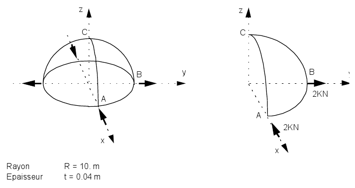
SSLS105	Title: Double pinched hemisphere. V Documentation: [] Models: SSLS105A DKT SSLS105B COQUE_3D MEC3QU9H

SSLS107	Title: Cylindrical panel subject to its own weight. V Documentation: [] Models: SSLS107A COQUE_3D MEC3QU9H SSLS107B COQUE_3D MEC3TR7H

SSLS108	Title: Helical shell under concentrated loads. V Documentation: [] Modelings: ;; SSLS108A COQUE_3D MEC3QU9H SSLS108B COQUE_3D MEC3TR7H ;;Notes: ** Use not recommended with DKT/DKQ, without transverse shears.







Ssls120: pressure cylinder	This test shows that triangle meshes are much more sensitive than quadrangle meshes. Triangle mesh with amplified deformity Quadrangles mesh with amplified deformity

Other test cases are described more briefly in the following table:

Name	Model	Remarks
HPLA100A HPLA100B HPLA100C HPLA100D HPLA100E hpla100f	2D_AXIS COQUE_AXIS COQUE_3D COQUE_3D COQUE COQUE	Title: Thermoelastic hollow cylinder weighing in uniform rotation. V documentation: [V7.01.100] The purpose of this test is to test the second members corresponding to the effects of gravity and to an acceleration due to a uniform rotation. Analytical solutions for the COQUE_3Dincluent metric variation in shell thickness. Analytical solutions for plates do not have metric corrections.
HSLS01A hsls01b	DKT/DST /Q4G COQUE_3D	Title: Embedded thin plate subjected to a thermal gradient in thickness. V documentation: [V7.11.001]
hsns100a hsns100b	COQUE_3D/DKT COQUE_3D/DKT	Title: Plate subject to a temperature gradient in thickness. V documentation: [V7.23.100] This test case makes it possible to test two ways of imposing the thermal field. The results obtained in a and b must be identical, but the reference solutions obtained are numerical.
SSLS114A SSLS114B SSLS114C SSLS114D ssls114i	COQUE_3D COQUE_3D DKT/DST DKQ/DSQ COQUE_AXIS	Title: Pressurization of a quarter of a cylindrical shell. V documentation: [V3.03.114] Analytical reference solution. Allows you to test the pressure term and the orientation of the normals. We test the results in radial displacement and in radial stresses.

2.5.2. Modal analysis in dynamics#

Name	Model	Remarks
SDLS01A SDLS01B SDLS01C SDLS01D SDLS01E SDLS01F SDLS01G sdls01h	DKT DKT DKT DKT COQUE_3D COQUE_3D COQUE_3D COQUE_3D	Title: Thin square plate free or embedded on one edge V documentation: [V2.03.001] It is a modal calculation and a harmonic response calculation. For modal calculation, it is a question of calculating the natural modes of bending of a thin square plate that is free or embedded on an edge. a - Edges of the plate oriented along the axes of the coordinate system. b - Any orientation of the plate and harmonic response for the embedded plate. c - Modal calculation by classical and cyclic dynamic substructuring. d - Modal calculation following a Guyan substructuring. e - Edges of the plate oriented along the axes of the coordinate system. f - Edges of the plate oriented along the axes of the coordinate system. g - Any orientation of the plate and harmonic response for the embedded plate. h - Any orientation of the plate and harmonic response for the embedded plate. * For a and b, the accuracy on the natural frequencies is less than 1% up to the sixth mode of bending * For c in substructuring, the quality of the results can be improved by using a finer substructure mesh. * For d, in order to obtain a precision of 1% on the natural frequencies, it is necessary to also condense on the nodes in the middle of the edges. * For e, f, g and h, the precision on the natural frequencies is less than 1% up to the sixth mode of bending for quadrangle elements and less than 2% for triangle elements. The shell element MEC3QU9Hest performs well compared to the element DKTqui is itself more efficient than the element MEC3TR7H.
sdls109a sdls109b, c sdls109d, e	DKQ (MEDKQU4) and DSQ (MEDSQU4) DKT (MEDKTR3) and DST (MEDSTR3) COQUE_3D (MEC3QU9H and MEC3TR7H)	Title: Natural frequencies of a thick cylindrical ring. V documentation: [V2.03.109] This test is inspired by a vibratory study carried out on collector VVP of N4 slices. This collector is thick and has a maximum thickness to mean radius ratio of 0.13. This value, which may be typical of an industrial structure, is slightly higher than the validity limit value usually recognized for plates and shells. In this study, the modeling of the collector in shells is then evaluated by comparison with a volume model on a ring. This test makes it possible to evaluate the algorithm for finding eigenvalues CALC_MODES [U4.52.02] with the stiffness and mass matrices.

2.5.3. Nonlinear static analysis (material)#

SSNL501	Title: Embedded beam subjected to uniform pressure. V Documentation: [] Models: SSNL501E COQUE_3D MEC3QU9H SSNL501D COQUE_3D MEC3TR7H SSNL501B DKT SSNL501C DKQ

Other test cases are described more briefly in the following table:

Name	Model	Remarks
SSNP15A SSNP15B SSNP15C ssnop15d	3D C_PLAN DKT COQUE_3D	Title: Square plate in tension-shear - Von Misès (isotropic work hardening). V documentation: [V6.03.015] A plate, made of a plastic material with linear isotropic work hardening, is subjected to a tensile force and a shear force. Even if the test validates the law of behavior rather than the elements to which it applies, it allows you to test the values of stresses, forces and deformations in the frame defined by the user (ANGL_REP).
SSNV115A SSNV115B SSNV115C SSNV115D ssnv115e	D_PLAN DKT DKT COQUE_3D COQUE_3D	Title: Corrugated sheet metal in non-linear behavior. V documentation: [V6.04.115] This test validates nonlinear behaviors in thin plate or shell models. Modeling A (2DD_PLAN) is used as a reference. The values of the trips are tested.

2.5.4. Geometric nonlinear static analysis#

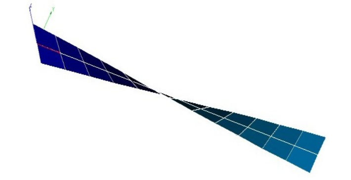
SSNV138	Title: Cantilever plate in large rotations subjected to a moment. V Documentation: [] Modelings: ;; SSNV138 COQUE_3D MEC3QU9H SSNV138 COQUE_3D MEC3TR7H ;;Note: ** The largest rotation achieved is slightly less than. The results obtained are very satisfactory, the maximum difference is less than 0.01%. It is necessary to increase the value of COEF_RIGI_DRZ (10E-5 by default) to 0.001 in order to be able to increase the value of the rotation angle that can be reached.

SSNV139	Title: Bias plate. V Documentation: [] Models: SSNV139 COQUE_3D MEC3QU9H SSNV139 COQUE_3D MEC3TR7H

SSNL502	Title: Beam in buckling. V Documentation: [] Models: SSNL502 COQUE_3D MEC3QU9H SSNL502 COQUE_3D MEC3TR7H

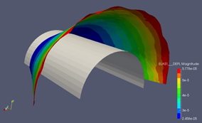
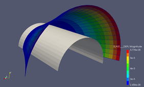
SSNS501	Title: Large displacements of a cylindrical panel. V Documentation: [] Models: SSNS501 COQUE_3D MEC3QU9H SSNS501 COQUE_3D MEC3TR7H

Other test cases are described more briefly in the following table:

Name	Modeling	Notes
SSNV140A ssnv140b	COQUE_3D COQUE_3D	Title: Recessed cylindrical panel subjected to surface force. V documentation: [V6.04.140] This force is constant for modeling a and is constant in modeling b. The aim of this test case is to verify the COQUE_3Dnon -linear geometric modeling using the algorithm for updating large 3D rotations GROT_GDEPde STAT_NON_LINEet to verify the treatment of the following pressures. The data for this problem corresponds to a thin shell \(h\mathrm{/}L\mathrm{=}0.625\text{\%}\), which is severe for the finite element triangle MECQTR7H (case of transverse shear blocking).
ssnv141a	COQUE_3D	Title: Title: Pinched spherical cap. V documentation:** [V6.04.141] The data for this problem corresponds to a thin shell \(h\mathrm{/}L\mathrm{=}0.4\text{\%}\), which is severe for the finite element triangle MECQTR7H (case of transverse shear blocking). It is necessary to increase the value of COEF_RIGI_DRZqui assigns a stiffness around the normal of the shell elements which by default is \({10}^{\mathrm{-}5}\) the lowest flexural stiffness around the directions in the plane of the shell in order to be able to increase the value of the angle of rotation that can be achieved. Values of this coefficient up to \({10}^{\mathrm{-}3}\) remain legal.
ssnv144a	COQUE_3D	Title: Title: Elbow in plane, elastic, flexible, embedded on one side and subjected to a linear force equivalent to a bending moment. V documentation:** [V6.04.144] The aim of this test case is to verify that, for elements COQUE_3D, the quasistatic solutions in geometric linear (VMIS_ISOT_LINEdans STAT_NON_LINE) and in geometric nonlinear (GROT_GDEPdans STAT_NON_LINE) are close to the linear static solution (MECA_STATIQUE) in the field of small disturbances.
SSNV145A ssnv145b	COQUE_3D COQUE_3D	Title: Cantilever plate in large rotations subjected to successive pressure. V documentation: [V6.04.145] The aim of this test case is to verify modeling COQUE_3D (mesh TRIA7, QUAD9) in the presence of a follower type of pressure.

2.5.5. Euler buckling analysis#

SSLS110	Title: Stability of a compressed square plate. V Documentation: [] Models: SSLS110 COQUE_3D MEC3QU9H SSLS110 COQUE_3D MEC3TR7H SSLS110 DKT MEDKQU4 SSLS110 DKT MEDKTR3

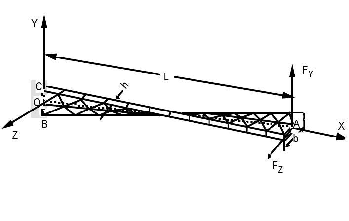
SDLS504	Title: Lateral buckling of a beam (spill). V Documentation: [] Models: SDLS504 COQUE_3D MEC3QU9H SDLS504 COQUE_3D MEC3TR7H

SDLS505	Title: Buckling of a cylindrical envelope under external pressure. V Documentation: [] Models: SDLS505 COQUE_3D MEC3QU9H SDLS505 COQUE_3D MEC3TR7H SDLS505 DKT MEDKTR3 SDLS505 DKT MEDKQU4

2.5.6. Connections, shells and other mechanical components#

SSLX100	Title: 3D-Hull-Hull-Bending Beam Mix. Documentation V: [] Modelings: ** SSLX100A 3D 1 MECA_HEXA20 DKT 4 MEDKTR3 POU_D_E 2 POU_D_E SSLX100B 3D 1 MECA_HEXA20 DKT 4 MEDKTR3 POU_D_E 2 POU_D_E We test the arrows, stresses, axial deformations and bending moments at 4 points on the axis of the beam.

SSLX102

Title: Piping bent during bending.

V Documentation: []

Models:

SSLX102A        DKT et TUYAU

(liaison COQUE_TUYAU)

SSLX102D        COQUE et POUTRE

SSLX101A

Title: Straight pipe modelled in shells and beams [].

V Documentation: []

Models:
SSLX101A        DIS_TR            POI1
DKT                MEDKQU4
POU_D_E        2 SEG2
Embedding the shell on the edge \(\mathit{P1}\). Flexion and traction in \(\mathit{x1}\). Difference of 3 to 5% on movements and rotations in \(\mathit{P2}\) with the analytical solution, due to the shell mesh with plane elements.
SSLX101B        DKT            MEDKQU4, METUSEG3
TUYAU        METUSEG3, MEDKQU4
DIS_TR        POI1
This modeling aims to test the shell-pipe connection in the presence of unit loads: traction, bending and twisting. The reference solution is analytical (RDM). The difference with the numerical solution is explained by the fact that the shell mesh is actually made up of plane elements (facets). The geometry of the pipe is therefore itself approximated.
SSLX102A        DKT            MEDKQU4, METUSEG3
TUYAU        MEDKQU4, METUSEG3
Modeling A involves the shell_pipe connection, the solution obtained (\(2.7\text{\%}\) difference in plane flexure, and \(0.4\text{\%}\) in out-of-plane flexure, with respect to the reference: all-shell mesh (modeling D) makes it possible to test the proper functioning of the connection between shell and pipe.

SSNs115a

Swelling of a flexible membrane

The objective of this test is to validate the functioning of the element MEMBRANE in large deformations for two hyperelastic laws of behavior and different types of cells (linear, quadratic and bi-quadratic). The swelling of a disk subjected to a subsequent pressure is therefore considered and the results are compared with solutions drawn from the literature.

Ssls108

Test taking into account a physical rotation around normal COEF_RIGI_DRZ =-1.E-8.