2. Method SRM

2.1. Generality of the SRM method

The SRM method takes advantage of relevance and loyalty, and this, to the reality of the finite element method to analyze stability slopes without the need to assume sliding circles in advance. In fact, using the Mohr-Coulomb or Drucker-Prager failure criterion, method SRM defines the safety factor as the relationship between the initial material parameters and the reduced parameters leading to discrepancy of the non-linear calculation under the static loads apply:

(2.1)\[ \ mathit {FS} =\ frac {c} {{c} {c} _ {i}} =\ frac {\ mathrm {tan} (\ varphi)} {\ mathrm {tan} ({\ varphi} _ {i})}} =\ frac {\ mathrm {i})} =\ frac {\ mathrm {tan} ({\ psi} _ {i})} =\ frac {\ mathrm {tan} ({\ psi} _ {i})} =\ frac {\ mathrm {tan} ({\ psi} _ {i})}\]

where

• \(\psi\) is the angle of expansion of the material

• \(c\) and \(\varphi\) represent cohesion and angle respectively of friction of the material composing the embankment.

Griffiths et al. [1] show that the expression (2.1) has the same physical meaning as the traditional definition by the ratio between the resistance force and the tangential force along the fracture surface.

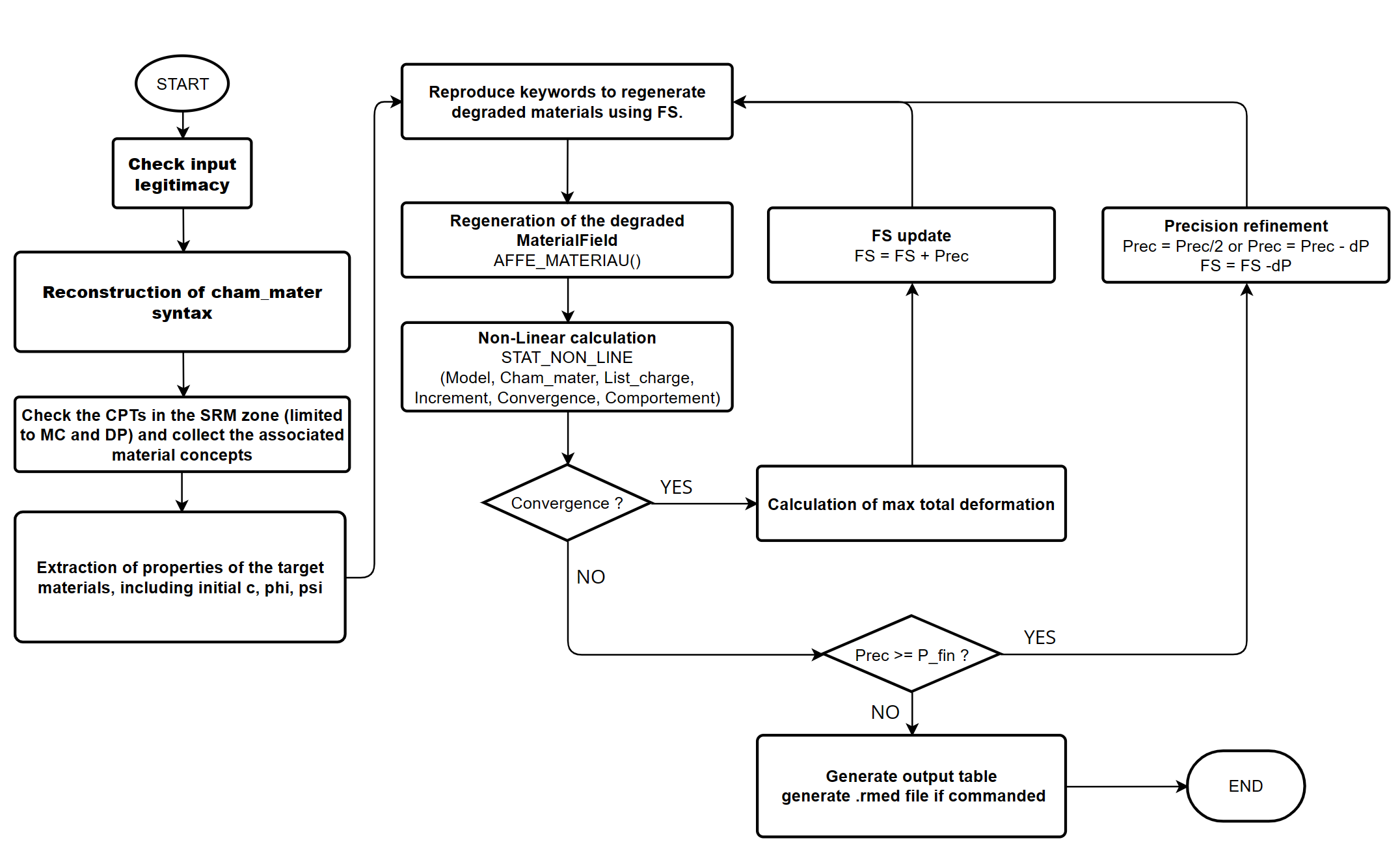
As illustrated in fig1-srm, computer processing in command CALC_STAB_PENTE from method SRM is done in 3 steps:

• Step 1: Treatment of zone SRM. Existing materials are identified

  in the zone SRM indicated, and the cell groups are created in the zone SRM in order to reallocate the field of degraded materials.

• Step 2: Creation of the degraded materials field. We then test

  the convergence of the nonlinear calculation and we refine the increment of the safety factor until the calculation diverges and the desired precision is reached.

• Step 3: Post-treatment. If requested, the deformation field is obtained at the output

  cumulative plastic (V1 of field VARI_NOEU) in order to visualize the fracture surface.

2.2. Treatment of zone SRM

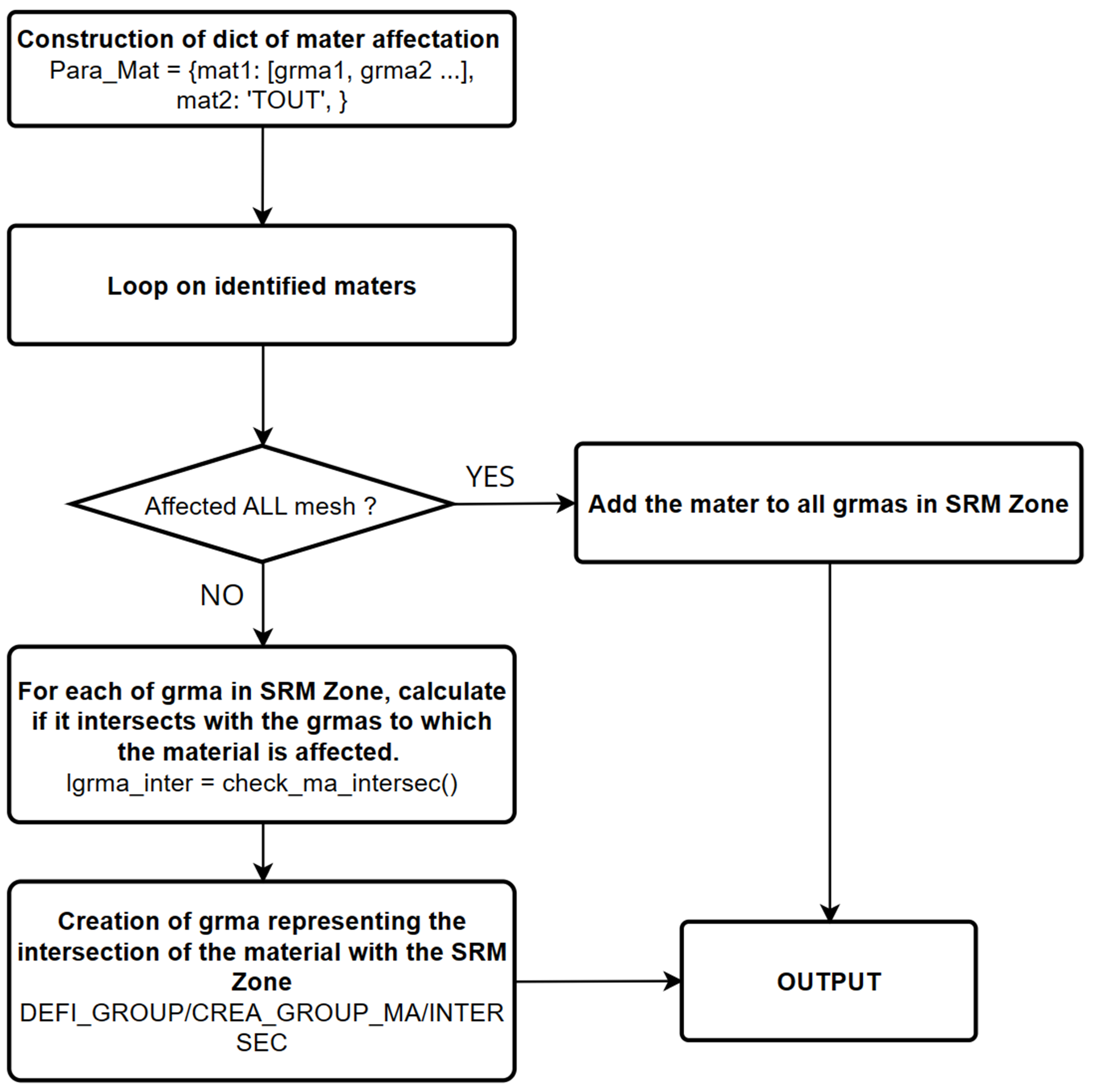
The CALC_STAB_PENTE command defines the zone where the SRM algorithm applies. This feature is particularly suitable when the model includes several slopes and we want to check the stability of a slope that is not necessarily subject to the greatest risk of breakage. Note that zone SRM can be defined by the mesh groups distinct from those that apply in the field assignment input materials. In this case we identify the materials in zone SRM and the cell groups are reassigned by the principle of overload.

As illustrated by fig2-srm-mater, for each group of In zone SRM, we check if it has meshes in common with the groups of meshes affected by the materials present in the aster object cham_mater.

2.3. Reduction in the strength properties of materials

The Mohr-Coulomb and Drucker-Prager failure criteria are allowed in CALC_STAB_PENTE. At the same time as generating the field of degraded materials, We check that there is exactly one law of behavior among both assigned to zone SRM by the keyword factor COMPORTEMENT.

Based on expression (2.1), degraded properties are calculated by:

(2.2)\[ \ mathrm {tan} (\ varphi\ text {'}) =\ frac {\ mathrm {tan} (\ varphi)} {\ mathit {FS}}},\ text {} c\ text {'} =\ frac {c} {\ mathit {FS}},\ text {} c\ text {'}}\]

We hypothesize the plastic flow law associated with Mohr-Coulomb behavior, be \(\varphi \text{'}=\psi \text{'}\). Otherwise, the angle of dilatance will take automatically the value of the friction angle when running algorithm SRM.

Apart from the Mohr-Coulomb criterion, it is also possible to use the criterion Drucker-Prager that improves the singularity problem caused by cone vertices of the Mohr-Coulomb charge surface in plane \(\pi\). Instead of reducing the Drucker-Prager settings directly (\(\mathrm{\alpha }\)) and \({\sigma }_{y}\)), the command favors the phi-c strategy to avoid the conservatism of the result [3]:

(2.3)\[ \ mathrm {tan} (\ mathrm {\ varphi}\ text {'}) =\ frac {3\ mathrm {\ alpha}} {2\ mathit {FS}\ sqrt {(2\ mathrm {\ varphi} +1) (2\ mathrm {\ alpha}} +1) +1) (1-\ mathrm {\ alpha} +1) (1-\ mathrm {\ alpha})}}, c\ text {'} =\ frac {{\ mathrm {\ mathrm {\ alpha} +1) +1) (1-\ mathrm {\ alpha} +1) (1-\ mathrm {\ alpha})}}, c\ text {'}} =\ frac {{\ mathrm {\ mathrm {\ alpha} +1) sigma}} _ {y}} {2\ mathit {FS}\ sqrt {(2\ mathrm {\ alpha} +1) (1-\ mathrm {\ alpha})}},\ mathrm {tan}\ mathrm {\ tan}\ mathrm {\ FS}\ mathrm {\ tan}}} {\ mathit {FS}} {\ mathit {FS}}}\]

2.4. FS convergence control

In order to speed up the search for the safety factor (FS), it is possible to control iterative resolution by configuring parameters related to refinement by increment \(\mathit{dP}\) (fig1-srm) according to the method indicated. The increment decreases each time the nonlinear calculation diverges until the maximum residue be reached.

Two laws of variation of increment \(\mathit{dP}\) are available:

1. “ EXPONENTIELLE “: Exponential change

The safety factor increment approaches the maximum residue exponentially. At the n^e refinement, the increment is calculated by:

\[\]

: label: eq-4

{p} _ {n} = {p} _ {0} {2} ^ {-n}

until \({p}_{N}<{p}_{\mathit{fin}}\), where

• \({p}_{n}\) is the current increment

• \({p}_{0}\) is the initial safety factor increment.

1. “ LINEAIRE “: Linear variation

The safety factor increment approaches the maximum residue linearly. In this case an additional ITER_RAFF_LINE operand is required. At the n^e refinement, the increment is calculated by:

\[\]

: label: eq-5

{p} _ {n} = {p} _ {0} -nfrac {{p} _ {0} - {p} _ {mathit {fin}}} {0}} {N}

until \({p}_{N}={p}_{\mathit{fin}}\).

Note

The advantage of the exponential method is that the calculation converges more quickly, while the linear method better controls the accuracy of the result. The exponential variation of the increment is especially adapted to the calculation with big INCR_INIT.

The following method would simplify the choice between the two laws of variation of the increment. Let \(N\) be the desired number of refinements, we choose the linear law if:

(2.4)\[ \ frac {{p} _ {0} - {p} - {p} _ {\ mathit {log}}} {{\ mathrm {log}}} _ {2} ({p} _ {0}) - {\ mathrm {log}}} _ {2} ({p} _ {\ mathit {end}})} <N\]

In these cases, the exponential law is chosen.