3. Method LEM

3.1. Generality of the LEM method

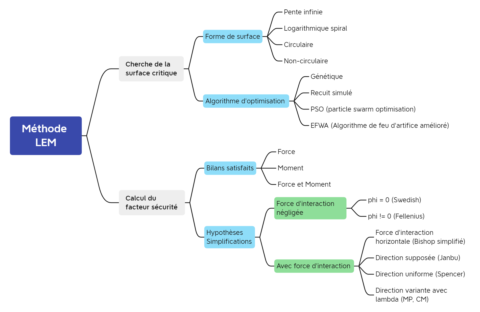
All methods like LEM are based on the definition of the safety factor as being the ratio between shear strength and tangential force along the fracture surface.

By dividing the slope into slices, which are considered to be non-deformable solids, We solve the balance of forces and moments of each bracket to to derive/to establish the safety factor. By respecting this principle of common calculation, the various methods LEM are distinguished by the number of satisfied reviews and the hypotheses on the strength of interaction between the slices.

A general overview of limit equilibrium resolution methods is given in fig4-lem2. 4 LEM methods are available in CALC_STAB_PENTE, adapted to the analysis of slopes with fracture surfaces both circular and non-circular:

• Simplified Bishop method and Fellenius method: These are the most common methods

  classics that assume that the fracture surface is circular.

  Thanks to rotational sliding, the number of equilibrium equations at the moment is reduced, which is equal to the number of slices, in an equation describing the equilibrium at the moment of the entire sliding part. Thus, the safety factor is calculated in a simple way using an explicit expression (Fellenius) or by an implicit scalar equation (Bishop).

• Spencer method and Morgenstern-Price: These are the most common methods

  conventional ones assuming that the fracture surface is non-circular.

  We solve all the equilibrium equations, whose quantity is equal to 3 times the number of slices, in order to obtain the most accurate safety factor result possible. The resolution procedure is becoming more sophisticated, which makes it possible to obtain a result more accurate if the fracture surface is visually non-circular.

---

In addition, since methods LEM do not rely on a finite element calculation, the optimization algorithms implemented in CALC_STAB_PENTE are essential to identify the fracture surface that minimizes the safety factor overall:

• Exhaustion method for the circular surface: We go through all

  the combinations of the end points of the potential fracture surfaces. This is the method implemented in most geotechnical software. commercial ones such as SLOPE /W by GeoStudio [8].

• Improved fireworks algorithm (EFWA) for the non-circular surface [4]:

  It is an intelligent swarm algorithm that is inspired by the process of generating sparks when fireworks explode. It is more efficient than other algorithms to optimize the numerical efficiency of solving the problem of slope stability with non-circular fracture surface [5].

One of the particularities of implementing methods LEM is that we calculate the weight of the slices using the same mesh used for finite element calculation. Although this requires mesh optimizations, developed in the command (in order to avoid slowing down at best the resolution of the safety factor) the advantage is reflected in the fact that we will no longer need to switch between solvers/models to perform the various types of analysis of an embankment structure.

For example, it is possible to directly combine the calculation of the interstitial pressure field due to water infiltration and slope stability analysis.

3.2. Calculation of the forces and geometry of the slices

In order to solve the balance of strengths and moments of the slices, First of all, it is necessary to calculate the geometric parameters defining the part slippery from the ground, and then calculate their own weight and possibly the pore pressure at the base of the slices.

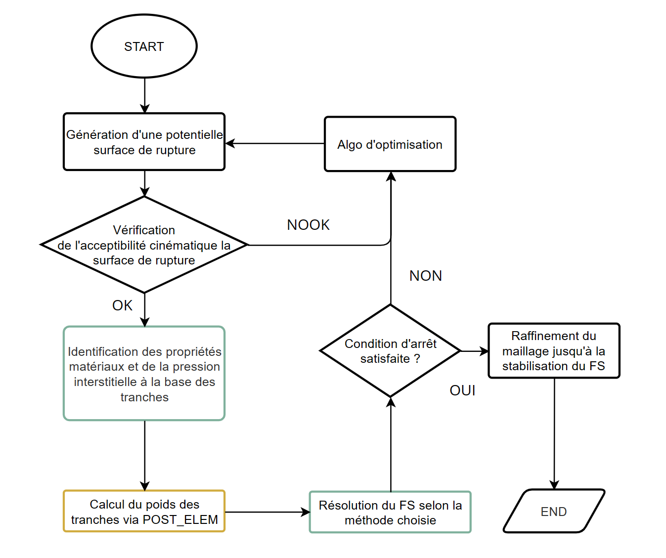
fig5-fs-tranche shows the overall workflow for retrieving information intervals required to calculate the safety factor later.

3.2.1. Calculating the center of the sliding circle

In case of a circular break surface, in order to create the mesh group Of the sliding part, we find the coordinates of the center of the sliding circle in two ways:

1. With endpoints and radius as inputs:

   By injecting the coordinates of the endpoints (\(({x}_{1},{y}_{1})\)) and \(({x}_{2},{y}_{2})\)) in the equation of the circle, we get the equations expressing the relationship between the coordinates of the center \(({x}_{0},{y}_{0})\) and a second-order equation from \({y}_{0}\):

   where the constants \({c}_{1}\) and \({c}_{2}\) are written:

   To solve equation eq-7, we express the coefficients in the second equation as:

   So we get the ordinate of the center. Since the fracture surface is always convex, we take the biggest solution:

2. With endpoints and a tangential horizontal line as inputs:

   In the case where the search for the critical radius is controlled manually by the operands Y_ MINI and Y_ MAXI from CALC_STAB_PENTE, we deduce the center of the circle from The \({y}_{b}\) ordinate of the tangential horizontal line.

   So you have to replace \(R={y}_{0}-{y}_{b}\) in equation eq-7 and repeat the same resolution procedure.

3.2.2. Creation of brackets and calculation of own weights

The slice cell group is created using the DEFI_GROUP operator by following the following steps:

• Step 1: Creation of the mesh group for the sliding part by the option “APPUI”

  with the nodes strictly included in the sliding surface.

• Step 2: Create the mesh group for slice \(n\) using the “INTERSEC” option

  which makes it possible to recover the common meshes of the abscissa band of the slice and the sliding part.

• Step 3: Correction of slice \(n\) with the “DIFFE” option

  which allows you to exclude cells belonging to the previous bracket. This step ensures that the total mass of the slices is equal to the mass of the sliding part.

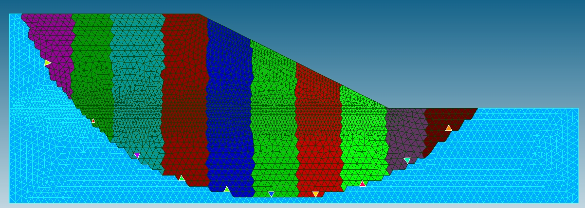
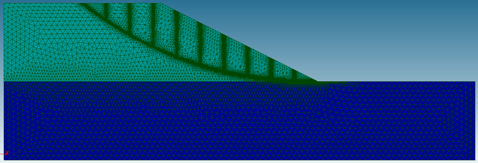
An example of mesh groups is shown in fig6-grma. The self-weights of the slices are then calculated using the operator POST_ELEM.

At the same time, the angle of inclination \(\alpha\) of the base of the slices is calculated. For the circular fracture surface, this angle is related to the derivative From the equation of the circle at the center of the base \(({x}_{c},{y}_{c})\):

(3.1)\[ \ mathrm {tan} (\ alpha) =\ frac {{x} _ {x} _ {c} - {x} _ {0}} {\ sqrt {{R} ^ {2} - {({x} _ {2}} - {c} _ {c} _ {c}} - {x} _ {0}})} ^ {2}}} - {({x} _ {2}} - {2}} - {x} _ {2}} - {2}} - {(x} _ {c}} - {c} - {x}}\]

For the non-circular surface, this angle is linked to the slope of the base of the slices:

(3.2)\[ \ mathrm {tan} (\ alpha) =\ frac {{y} _ {n+1} - {y} _ {n}} {{x} _ {n+1} _ {n+1}} - {x} _ {n}}\]

3.2.3. Material properties and pore pressure

The materials field at the input of the CALC_STAB_PENTE order makes it possible to regain cohesion and the angle of friction along the fracture surface. Behavioral parameters Drucker-Prager are converted by the same formula as () considering \(\mathit{FS}=1\).

It is assumed that the properties are homogeneous on the basis of each slice, and equal to those of the material affecting the mesh that contains the center of the base. This « center » mesh is defined by the criterion of minimum distance between the center of the mesh and the center of the base of the slices.

If necessary, the interstitial pressure is introduced using the control variable PTOT: of the material field, which is defined on the nodes of the elements. So we calculate the pressure at the center of the base via reverse remote interpolation (IDW):

(3.3)\[ u=\ frac {\ sum _ {i=1} ^ {1} ^ {N} {N} {(\ frac {1} {1} {d} _ {i}})} ^ {u} _ {i}} {\ sum _ {i}}} {\ sum _ {i}}} {\ sum _ {i}}} {\ sum _ {i}}} {\ sum _ {i}}} {\ sum _ {i=1}} ^ {i=1}} ^ {i=1}} ^ {i=1}} ^ {i=1}} ^ {i=1}} ^ {i=1}} ^ {i=1}} ^ {i=1}} ^ {i}}\]

where

• \({d}_{i}\) refers to the distance between the nodes of the mesh and the center of the base

• \({u}_{i}\) is the pressure at the knots.

3.3. Circular fracture surface

3.3.1. FS calculation using Bishop or Fellenius methods

1. Fellenius method

The Fellenius method is also called the « Swedish method » or « ordinary method of slices » [2]. This method completely neglects the strength of interaction between the slices. So the FS formula becomes explicit. The force diagram is shown in fig7-fellenius.

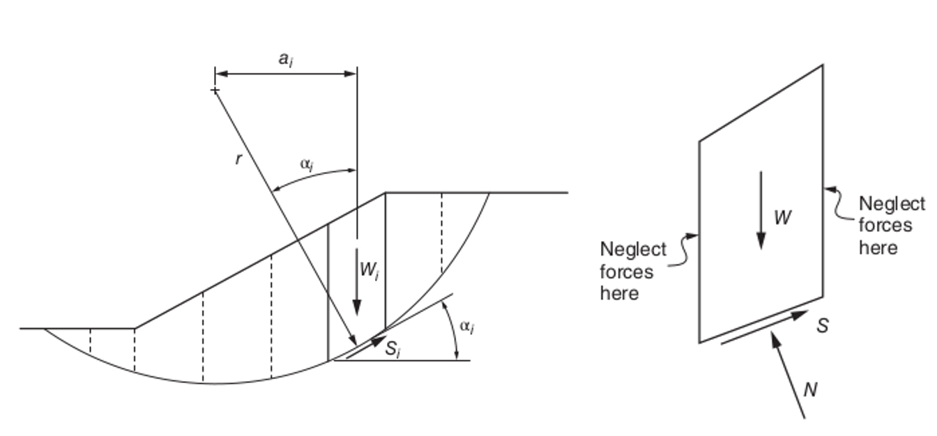
With the presence of interstitial pressure, the normal force on the base of the slices is written as:

(3.4)\[ N\ text {'} =W\ mathrm {cos}\ alpha -u\ mathrm {\ Delta} l {\ mathrm {cos}}} ^ {2}\ alpha\]

where

• \(W\) refers to weight,

• \(u\) refers to interstitial pressure,

• \(\mathrm{\Delta }l\) is the length of the base.

Depending on the equilibrium at the moment of the sliding part in relation to the center of the sliding circle, the safety factor is expressed by:

(3.5)\[ \ mathit {FS} =\ frac {\ sum c\ mathrm {\ Delta} l+ (W\ mathrm {cos}\ alpha -u\ mathrm {\ Delta} l {\ mathrm {cos}}} ^ {cos}}} ^ {2}\ alpha} ^ {2}\ alpha)\ mathrm {2}\ alpha)\ mathrm {\ delta}\]

2. Bishop’s method simplified

The simplified Bishop method assumes that the force of interaction between the slices is horizontal, as shown in fig8-bishop-simple.

The balance of forces in the vertical direction is written as:

(3.6)\[ \ mathit {Ncos}\ alpha +S\ mathrm {sin}\ alpha -W=0\]

In addition, according to the Mohr-Coulomb criterion, the tangential resistance force is written as:

(3.7)\[ S=\ frac {1} {\ mathit {FS}}} [c\ mathrm {\ Delta} l- (n-U\ mathrm {\ Delta} l)\ mathrm {tan}\ varphi]\]

We therefore deduce the implicit expression of the safety factor:

(3.8)\[ \ mathit {FS} =\ dfrac {\ sum\ dfrac {c\ mathrm {\ Delta} l\ mathrm {cos}\ alpha + (w-u\ mathrm {\ Delta} l\ mathrm {cos}\ alpha)\ mathrm {cos}\ alpha)\ mathrm {cos}\ alpha + (\ mathrm {sin} l\ cos}\ alpha + (\ mathrm {sin}\ alpha}\ alpha mathrm}\ alpha mathrm {cos}\ alpha + (\ mathrm {sin}\ alpha}\ alpha mathrm {cos}\ alpha) thrm {tan}\ varphi)/\ mathit {FS}}}} {\ sum\ mathit {Wsin}\ alpha}\]

Equation :eq:`eq-18` is solved using the fixed point iteration method.

3.3.2. Critical surface location

In order to locate the critical surface, we go through all the possible combinations end points of potential fracture surfaces. For each combination, we increment the radius to find the circular area that minimizes the FS. The radius increment takes the value of 10% of the slope height. The illustrious fig9-surf-crit the critical surface search workflow

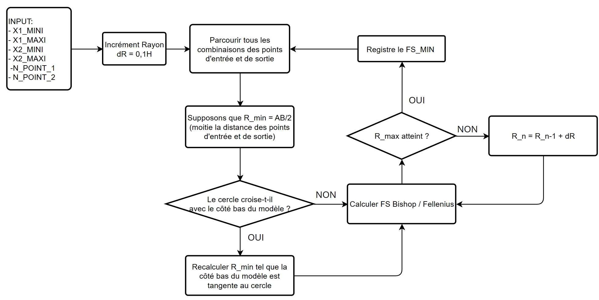
Two approaches are available to determine radius test bands:

• Option 1: We scan all the rays that form a kinematically admissible fracture surface.

  The upper limit is set by \({R}_{\mathit{max}}=\mathrm{1,5}{R}_{\mathit{pied}}\) where \({R}_{\mathit{pied}}\) is the radius of the circle tangential to the horizontal line through the lower end. The lower limit is the minimum value among:

  • Half the distance between endpoints.

  • The radius of the tangential circle at the base of the mesh.

• Option 2: The test strip is manually defined by defining the horizontal lines

  tangential to the fracture surfaces. This search option speeds up the calculation if the experienced user foresees the reduced zone where the fracture surface is likely to be located. We also take advantage of this option to examine the surfaces in the vicinity of that given by the result. If the limits of the ordinates Y_ MINI and Y_ MAXI are close, the radius increment is adapted so that at least 3 spokes are to be tested (an intermediate radius).

The radius increment equal to 10% of the height is sometimes too big to locate the critical surface in a precise manner. Faced with this problem, after calculating the safety factor corresponding to all the rays tested for a combination of end points, if a new minima appears, it is recorded by doing a local check of the radius. This check is done by iteratively refining the radius increment in order to exponential, and by testing the rays around the radius that minimizes the safety factor.

In iteration \(n\), the refined increment is written as:

(3.9)\[ {\ mathit {dR}} _ {n} = {2} ^ {-n} {\ mathit {dR}} _ {0}\]

We then test the rays:

(3.10)\[ {R} _ {n} = {R} _ {\ mathit {minFS}, n-1}\ pm {\ mathit {dR}}} _ {n}\]

During iterations, the minimizing radius is always recorded the safety factor and we continue to test its surroundings with the refined increment until the radius is stabilized.

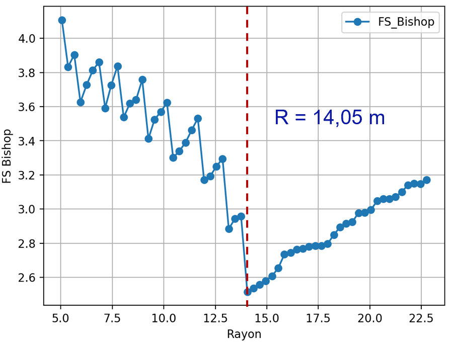
Based on tests, this optimization algorithm designed for circular surfaces proves to be effective even for inhomogeneous slopes. The fig10-rc show that with the slope modelled in the ssnop507 test case [V6.03.507], the algorithm successfully locates the radius minimizing the FS globally.

3.4. Non-circular fracture surface

3.4.1. FS calculation using Spencer or Morgenstern-Price methods

The Spencer and Morgenstern-Price methods are designed to analyze the stability of slopes whose fracture surface is of a more complex shape due to the inhomogeneity of the materials, such as the stratification of the foundation and the presence of a weak layer (test case ssnap006 [V6.03.006]).

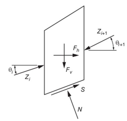
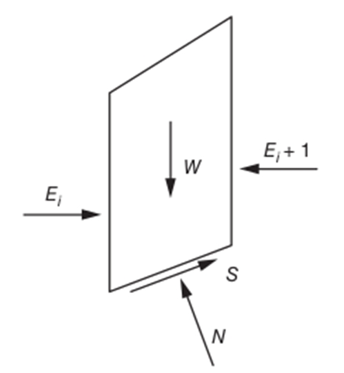
fig11-spencer-MP shows the diagram of the forces experienced by the slices when you choose the Spencer or Morgentern-Price method. \({F}_{v}\) refers to dead weight of the slice that is equal to \(W\) in equation (3.8). These methods satisfy all the equilibrium equations, which is \(n\) Equations for the balance of forces in the vertical direction, \(n\) in the horizontal direction and \(n\) moment equilibrium equations, where \(n\) is the number of slices. The two methods are distinguished by the hypothesis about the direction of forces of interaction between slices \({Z}_{i}\). We represent this direction by the angle \({\theta }_{i}\) with respect to the horizontal direction:

\[\]

: label: eq-21

mathrm {tan} ({theta} _ {i}) = {f} _ {i}) = {f} _ {i}) = {f} _ {1} ({x} _ {i}) +lambda {f} _ {i})

where \({f}_{0}\) and \({f}_{1}\) are the functions defining the variation of the angle of inclination of the interaction forces between the slices, and \(\lambda\) is a multiplying coefficient which is one of the unknowns of equilibrium equations. The functions \({f}_{0}\) and \({f}_{1}\) depend on the method chosen:

• Spencer method: \({f}_{0}=0,{f}_{1}=1\).

• Morgenstern-Price method (proposed by Chen and Morgenstern in 1983):

  • \({f}_{0}(x)=\mathrm{tan}{\beta }_{0}+\dfrac{\mathrm{tan}{\beta }_{1}-\mathrm{tan}{\beta }_{0}}{L}x\),

    where \({\beta }_{0}\) and \({\beta }_{1}\) are the angles of inclination of the slope profile at both extremities of the fracture surface.

  • \({f}_{1}(x)=\mathrm{sin}(\dfrac{\pi }{L}x)\)

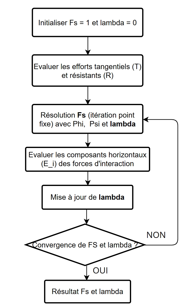
The safety factor resolution procedure proposed by Zhu et al. [6] is adopted. The advantage of this procedure compared to traditional procedures is that it deduces the pattern iterate the fixed point to calculate the safety factor and proposes a weak approach coupled to solve FS and \(\lambda\). According to the authors, this procedure of resolution is at the same time more efficient and effective than traditional procedures.

• The balance of force in the vertical direction of slice \(i+1\) is written as:

  where \({U}_{i}={u}_{i}\mathrm{\Delta }{l}_{i}\) represents total interstitial pressure applied to the base of the slice.

• The balance of force in the horizontal direction of slice \(i+1\) is written as:

By eliminating the normal force in the equations eq:eq-22 and eq:eq-23, we have the simplified balance of forces:

(3.11)\[ {Z} _ {i+1} {\ mathrm {\ Phi}}} _ {\ Phi}}} _ {\ Phi}} _ {i} {i} {\ mathrm {\ Phi}} _ {\ mathrm {\ Phi}}} _ {i}}} _ {i}} + {i} + {R} _ {i+1} - {F} _ {s} {T} _ {i+1}}\]

where

(3.12)\[\begin{split} \ begin {array} {c} {\ mathrm {\ Phi}} _ {i} = {F} _ {i} = {F} _ {i} = {F} _ {i} = {f} = {i}) +\ mathrm {sin} ({\ sin} ({\ alpha}} _ {s} _ {i})\ mathrm {tan} _ {i}) +\ mathrm {sin} ({\ sin}) ({\ alpha} _ {i})\ hfill\\ {\ mathrm {\ Psi}} _ {i} = [{F} _ {i} = [{F} _ {i}} = [{F} _ {i}) = [{f}} = [{i}) +\ mathrm {sin} ({\ sin}} ({\ sin}} ({\ alpha} _ {s}})\ mathrm {tan} _ {i}) +\ mathrm {sin} ({\ sin}} ({\ sin}) ({\ alpha} _ {i})\ mathrm {tan} _ {i}) +\ mathrm {sin} ({\ sin}} ({\ sin}} ({\ alpha} _ {i})\ mathrm {tan} _ {i}) +\ mathrm {sin} +1}]/{\ mathrm {\ Phi}}} _ {i}\\ {R} _ {i} = ({W} _ {i}\ mathrm {cos} {\ alpha} _ {i} - {U} _ {i})\ mathrm {tan} {\ varphi} {\ varphi} _ {i} _ {i}\ mathrm {\ delta}\ {i})\ mathrm {\ delta} l\ hfill\\ {T} _ {i} = {W} _ {i}\ mathrm {sin} {\ alpha} _ {i}\ hfill \ end {array}\end{split}\]

In fact, \({R}_{i}\) represents the shear strength generated by all the forces applied to the slice except the interaction forces between the slices. \({T}_{i}\) represents the driving force leading to the destabilization of the slice.

So, with conditions \({Z}_{0}={Z}_{N}=0\) (the interaction forces on both sides of the sliding part) are zero), we deduce the iteration scheme of the fixed point to calculate FS:

(3.13)\[ {F} _ {s} =\ frac {\ sum _ {i=1}} ^ {N-1} {R} _ {i}\ prod _ {j=1} ^ {N-1} {\ mathrm {\ Psi}} {\ mathrm {\ Psi}}} _ {j}}} _ {j}} + {J}} + {R} _ {N}} + {R} _ {N}}} {R} _ {N}}} {\ sum _ {i=1} ^ {N-1} {T} _ {i}\ prod _ {j=1} ^ {N-1} {\ mathrm {\ Psi}} _ {j} + {T} _ {N}}\]

Finally, the balance balance at the moment in relation to the center of the base of slice \(i+1\) is written:

\[\]

: label: eq-27

{E} _ {i+1} ({z} _ {i+1} +frac {b} {2}mathrm {tan} {alpha} _ {i+1}) = {E} _ {i} ({z}} ({z} _ {i} -frac {b} {i} -frac {b} {i}} -frac {b} {2}mathrm {tan} {alpha} _ {i+1}) = {E} _ {i}) +frac {b} {i} ({z} _ {i}) +frac {b} {i}) +frac {b} {i} {2} (mathrm {tan} {theta}} _ {i} {E} _ {i} +mathrm {tan} {theta} _ {i+1} {E} {E} _ {i+1})

where

• \({E}_{i}\) is the horizontal component of the interaction force that can be calculated using

  equation (3.11),

• \(b\) is the horizontal width of the slice,

• \({z}_{i}\) refers to the vertical distance between the point where the

  interaction force and the center of the base of the slices.

Let the moment of the horizontal component be in relation to the center of the Based \({M}_{i}={E}_{i}{z}_{i}\), we rewrite equation eq-27 as:

\[\]

: label: eq-28

{M} _ {i+1} = {M} _ {i} -frac {b} {i} -frac {b} {2}mathrm {tan} {alpha} _ {i} + {E} _ {i} + {E} _ {i+1}) +frac {b} {i+1}) +frac {b} {i+1}) +frac {b} {i+1}) +frac {b} {i+1}) +frac {b} {i+1}) +frac {b} {2} {2} [mathrm {tan} {theta} _ {i} {e} {e} {i} + {E} _ {i+1}) +frac {b} {i+1}) +mathrm {tan} {theta} _ {i+1} {E} _ {i+1}]

Taking into account condition \({M}_{0}={M}_{N}=0\), we deduce the expression for \(\lambda\):

(3.14)\[ \ lambda =\ frac {\ sum _ {i=1} {i=1} ^ {1} ^ {N} [\ mathrm {tan} {\ alpha} _ {i} + {E} _ {i+1}) - ({f} {i+1})) - ({f} _ {i+1}))) - ({f} _ {i+1}))) - ({f} _ {i+1}))) - ({f} _ {i+1}))) - ({f} _ {i+1}))) - ({f} _ {i+1}))}\ sum _ {i=1} ^ {N} ({f} _ {f} _ {1, i} {E} _ {i} + {f} _ {1, i-1} {E} {E} _ {i-1})}\]

We solve FS and \(\lambda\) by the alternative evaluation of its values to using equations (3.13) and (3.14) until the convergence of the two unknowns, as illustrated in fig12-FZ-spencer-MP.

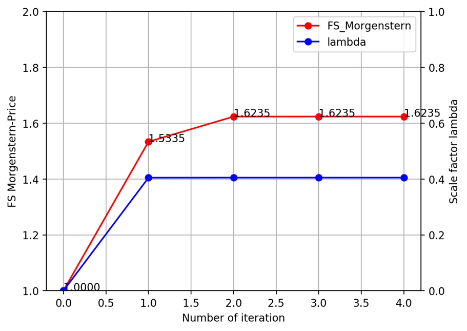
Based on the test results, this FS resolution procedure converges in two iterations, as shown in fig13-convergence-lambda.

3.4.2. Optimization algorithm EFWA

3.4.2.1. Optimization procedure

Due to the large number of state variables, the problem of surface location Non-circular criticism proves to be too difficult to be solved by the trial-and-error method. Recently, thanks to the emergence of intelligent swarm algorithms, many researchers use them to solve the problem of locating the non-circular fracture surface. For example, the particle swarm algorithm (PSO), the genetic algorithm, and the algorithm of ant colonies have shown their ability to find the optimum with an acceptable time cost.

Zheng et al. (2013) [4] proposed the improved fireworks algorithm (EFWA). Xiao et al. (2019) [5] first applied EFWA to slope stability analysis, and based on its results, EFWA achieves the optimum with less more iterations than other swarm algorithms [5].

In CALC_STAB_PENTE we therefore adopt EFWA as the optimization algorithm.

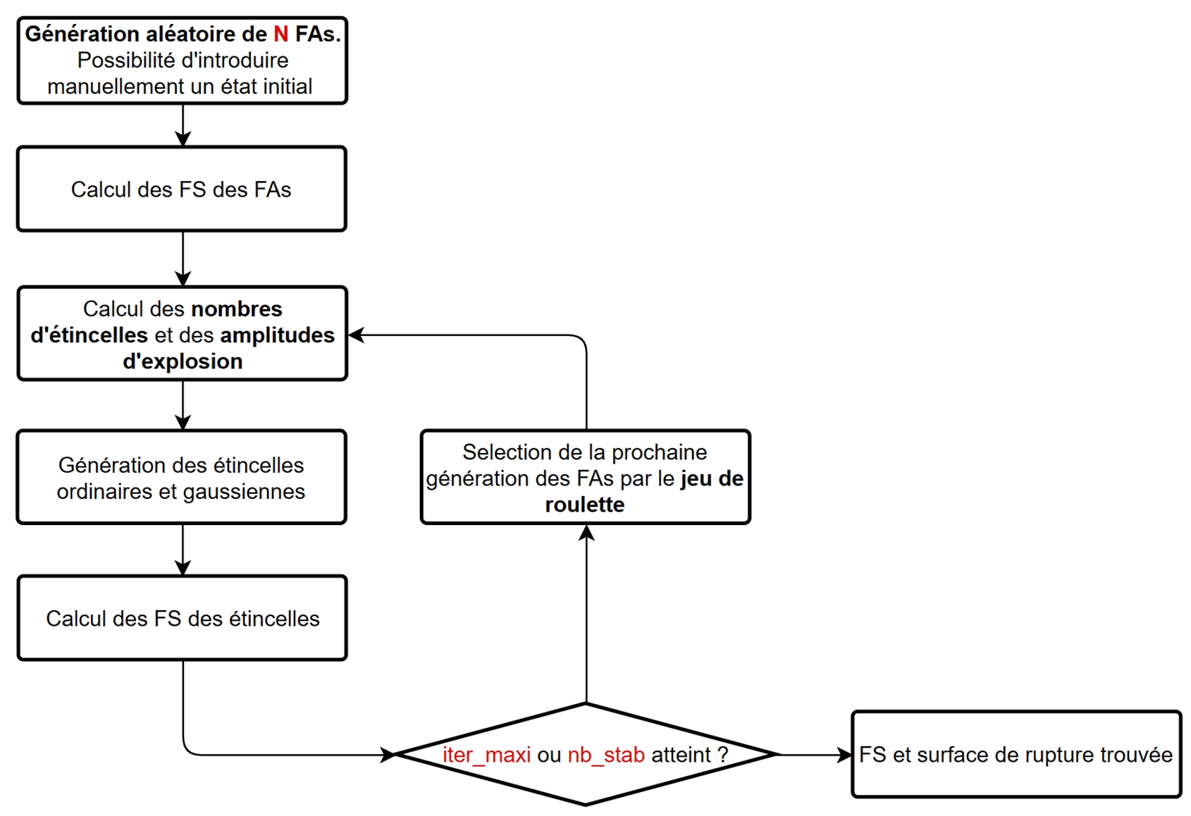
The EFWA simulates the process of fireworks exploding. In the space of state variables represented like the night sky, fireworks are detonated in various places. Each explosion locally generates sparks to search for the optimum in the neighboring space. Among these sparks, some that have significant selective value (inversely proportional to FS) are saved for the next explosion.

The EFWA takes place in 3 stages:

1. Random generation of the N initial fireworks

   The state variable vector has \(N+1\) components, or the abscissa of the end points of the break surface, and \(N-1\) ordinates of the intermediate points, where \(N\) is the number of slices:

   If the initial state is not specified via the ETAT_INIT operand of CALC_STAB_PENTE, We randomly generate \({N}_{\mathit{FA}}\) initial positions of the fireworks (uniform distribution law):

   where the limits of the degrees of freedom are determined by the algorithm described in section 3.4.2.2.

   If we provide operand ETAT_INIT, which is the output table for CALC_STAB_PENTE, it is added in the initial generation of fireworks.

2. Generation of ordinary and Gaussian sparks

   When generating ordinary sparks from explosion position \(i\), the amplitude of the explosion is calculated by:

   where \(A\) is the value of the A operand of CALC_STAB_PENTE designating the total amplitude of ordinary sparks, and \(ϵ=1e-8\) is a constant close to zero to avoid division by zero. With equation eq-32, we search in a larger amplitude if the central position is of inadequate quality, and we focus on the space near the positions close to of the minimum FS value.

   The number of ordinary sparks in an explosion is calculated by:

   where \(M\) is the value of the M operand of CALC_STAB_PENTE designating the total number of ordinary sparks. By equation eq-33 we generate more sparks if the central position is of good quality. In order to avoid the emergence of absurd numbers, we correct:

   Ordinary sparks are generated by arbitrarily modifying the degrees of freedom of the positions. of the current generation:

   In order to always maintain the diversity of the search for the optimum, Gaussian sparks of quantity \({M}_{g}\) are also generated. Firework positions are selected arbitrarily, and arbitrarily modified The degrees of freedom:

   where \({X}_{B}^{k}\) is the position corresponding to the minimum FS of the current generation.

   If some degrees of freedom are outside the limits determined by the algorithm described in section 3.4.2.2, they are projected into the allowable band:

   Because the modification of a degree of freedom influences the allowable band of intermediate points To the right of it, they are also adjusted so that the fracture surface generated is kinematically admissible.

   Finally, in case the fracture surface generated is so close to the slope profile that it is Impossible to create the group of the cells of the slices, we will correct the break surface so that it moves away from the slope profile:

   where \({X}_{\mathit{bc}}\) is the value of the MARGE_PENTE operand of CALC_STAB_PENTE.

3. Selecting sparks for the next generation

   The new generation of fireworks is happening through the roulette game algorithm. The probability that an ordinary or Gaussian spark will be retained in the next generation is:

Algorithm diagram EFWA is shown by fig14-diag-EFWA.

3.4.2.2. Dynamic constraints of state variables

: name: fig15-cont-varEtat

width:

70%

Illustration of the constraints of state variables

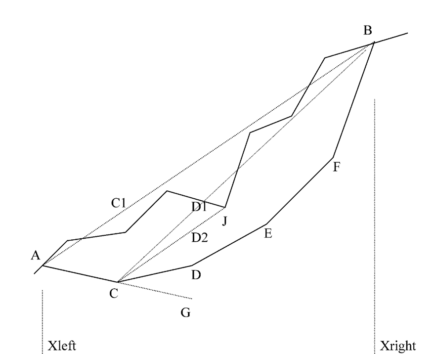
In order to ensure that the fracture surface is always convex and kinematically admissible, we adopt the procedure proposed by Cheng et al., for determining the constraints dynamics of state variables [7].

In this procedure, the ordinate limits of the intermediate points depend of one or two previous points (on the left). Let’s take the example in fig15-cont-VarEtat:

• Lower terminal:

  • The fracture surface being at a lower angle of 45 degrees with

    the slope profile at end point A, which determines the lower bound of point C.

  • We extend the line AC to the abscissa of point D to determine the lower bound of point D.

• Upper terminal:

  • We link CB and check if CB intersects with the profile

    of the slope. If they intersect, we find the intersection point with the minimum ordinate J and connect CJ to determine the upper bound D2 of the point D. Otherwise, D1 will be the upper bound of point D.

In order to ensure that the fracture surface remains in the model, the lower bound is adjusted at the bottom of the model if it is located below the latter.

3.5. Adapting the mesh

Since the stability analysis via CALC_STAB_PENTE is based on the mesh, the fineness of the mesh significantly influences the result of the safety factor. As a result, CALC_STAB_PENTE automates mesh refinement. However, the calculation time increases all the more the more the finer the mesh is. Therefore, as shown in fig16-sensibilite-maillage, we isolate the refinement of the critical surface search mesh, since the fineness of the mesh has a negligible influence on the location of the rupture surface.

In order to speed up the creation of slice groups, using the MACR_ADAP_MAIL command, we refine the mesh only on the contour of the slices until waiting for the maximum number of refinements or for the stabilization of FS. This process is driven by a proximity indicator field expressed under the form of a Gaussian function with zero mean and standard deviation \(\sigma\):

(3.15)\[ \ mathit {val} =\ frac {1} {\ sqrt {2\ pi}\ sigma}\ mathrm {exp} (\ frac {- {d} _ {\ mathit {min}}} {\ mathit {min}}}} ^ {min}}}} ^ {2}}} ^ {2}})\]

where \({d}_{\mathit{min}}\) is the minimum distance between a mesh node and the outline of the slices. We refine the knitwear according to the criterion of \(\sigma\), i.e. 68% of the meshes closest to the contour, and the meshes are de-refined according to the criterion of \(2\sigma\), or 5% of the stitches farthest from the outline.

We decrease the standard deviation exponentially to control dynamically the refinement zone.

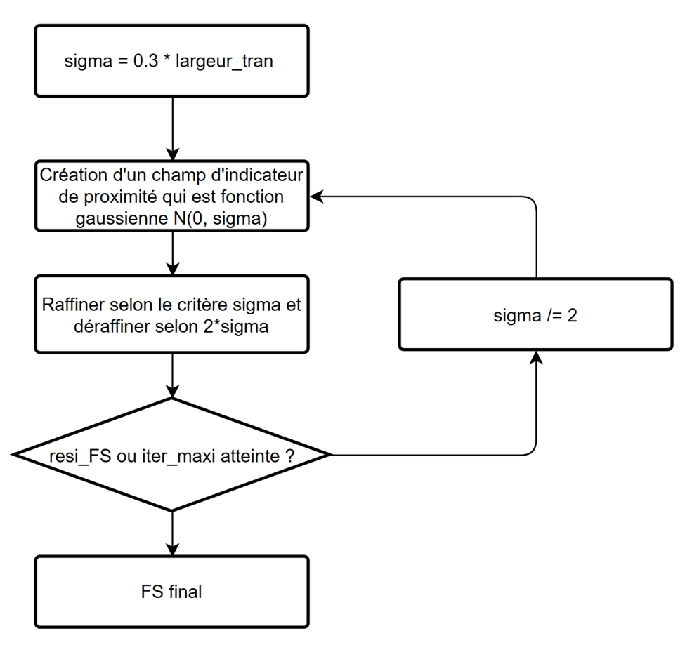
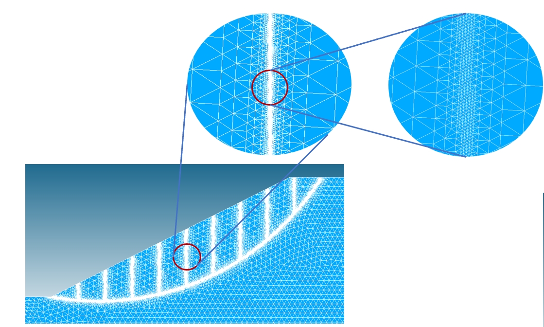
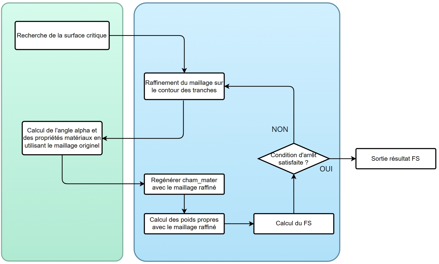
The fig17-algo-adapt-maillage illustrates the adaptation algorithm of the mesh and the result of the adapted mesh.