2. Stability of a dissipative system#
2.1. Definition of the stability of a dissipative system#
When we are interested in dissipative phenomena (case of plastic or fragile materials…) we add a term representing the part dissipated to the expression for total energy Φ. Irreversible degradations are then associated with quantities, most often scalar, such as damage or plasticity. The buckling criterion presented above does not take irreversibility into account. It is sufficient but not necessary to justify stability [bib19]. When the buckling criterion is reached, the uniqueness of the solution is no longer guaranteed, but it cannot be concluded directly about stability. We denote u the state variable deriving from the reversible part of the energy and α the state variable deriving from the irreversible part of the mechanical phenomenon studied. The stability criterion then consists in verifying the positivity of the second derivative of energy in the direction of the increase of the variable α [bib20]. Let us consider an admissible disturbance (qu, b≥0). The stability criterion then comes down to verifying that we always find the inequality:
\(\phi (u,\alpha )\mathrm{\le }\phi (u+v,\alpha +b)\) eq 2.1‑1
From a mathematical point of view, this is equivalent to verifying that the function Φ achieves a local minimum in (u, α).
We are particularly interested in the case of damage models. We consider (u, α), a state of the structure Ω verifying the balance:
\(\mathrm{\forall }v\mathrm{\in }{C}^{0},{\mathrm{\int }}_{\Omega }(\frac{\mathrm{\partial }\phi }{\mathrm{\partial }u}(u,\alpha )\mathrm{.}v)\mathit{dx}\mathrm{=}0\) eq 2.1‑2
and the damage criterion, taking into account the irreversibility of the state variable*α:*
\(\frac{\mathrm{\partial }\phi }{\mathrm{\partial }\alpha }(u,\alpha )\mathrm{\ge }0\mathit{et}\mathrm{\forall }\beta \mathrm{\in }{C}^{0}\mathrm{\ge }\mathrm{0,}{\mathrm{\int }}_{\Omega }(\frac{\mathrm{\partial }\phi }{\mathrm{\partial }\alpha }(u,\alpha )\mathrm{.}\beta )\mathit{dx}\mathrm{=}0\) eq 2.1‑3
We quickly obtain, with a Taylor expansion to order 2 [bib20], the equivalence between the criterion 2.1-1 and the following criterion, written on the second derivative of Φ:
\({D}^{2}\phi (u,\alpha )\mathrm{\ge }0\) eq 2.1‑4
where*D2* is the second derivative operator.
2.2. Writing in the framework of the finite element method#
From the point of view of finite elements and maintaining the previous notations, this criterion is written as the positivity of the Rayleigh quotient under the following inequality constraints:
\(\mathrm{\forall }(v,b\mathrm{\ge }0)\mathrm{\ne }0\text{,}{Q}_{\mathit{rc}}\mathrm{=}\frac{{(v,b)}^{t}\mathrm{.}{K}^{T}(v,b)}{{(v,b)}^{T}\mathrm{.}(v,b)}\mathrm{\ge }0\) eq 2.2‑1
The most traditional way to verify that a function is positive is to calculate its minimum and ensure that it is positive. In the following part, we present the minimization algorithm under inequality constraints programmed in Code_Aster.
2.3. Optimization algorithm under inequality constraints#
Among the algorithms available in the literature, the one that has proven to be the most robust and also the simplest to program is the power method, to which is added, at each iteration, the projection of the degrees of freedom \(b\) onto all the positive values, in order to verify the unilateral constraint imposed [bib21]. The algorithm is built in two steps, as follows:
The power method is widely used in applied mathematics to find the maximum eigenvalues of a M matrix. A shift to the largest eigenvalue λm :N=* **λmid-M then makes it possible to search for the smallest eigenmodes. The algorithm is presented below in its initial form. Or, in the form used to find the maximum eigenvalue of a symmetric matrix A:
\(\begin{array}{c}\text{Soit}P\text{la projection d'un vecteur sur sa partie positive.}\\ \text{Initalisation :}{(v,b\mathrm{\ge }0)}_{0}\mathrm{/}\mathrm{\parallel }{(v,b\mathrm{\ge }0)}_{0}\mathrm{\parallel }\mathrm{=}1\text{.}\\ \text{Pour}k\mathrm{\ge }1\text{}\text{Faire :}\\ \text{}(w,c)\mathrm{=}A{(v,b)}_{k\mathrm{-}1},\\ \text{}{(v,b)}_{k}\mathrm{=}(w,P(c)),\\ \text{}{(v,b)}_{k}\mathrm{=}{(v,b)}_{k}\mathrm{/}\mathrm{\parallel }{(v,b)}_{k}\mathrm{\parallel }\\ \text{}\text{Si :}\mathrm{\parallel }{(v,b)}_{k}\mathrm{-}{(v,b)}_{k\mathrm{-}1}\mathrm{\parallel }<\epsilon \text{alors Fin}\\ \text{}\text{Sinon :}k\mathrm{=}k+1\\ \text{}\text{Fin Si}\\ \text{Fin Pour}\end{array}\)
Figure 2.3-a: Diagram of the algorithm for finding the maximum under constraint for an A matrix
Its reliability limit is around a thousand degrees of freedom. To overcome this limit and to be able to deal with industrial problems, we use the reduction method available in Sorensen [bib22], which consists in projecting the problem on a base made up of the n smallest eigenmodes of the structure. Taking this step into account, the algorithm is rewritten in the following way, where K is always the tangent operator, Q is the projection operator and B n the projection into the reduced space:
\(\begin{array}{c}\text{Réduction :}{K}^{T}\mathrm{=}{Q}^{T}{B}_{n}Q\\ \text{Initialisation :}{(v,b\mathrm{\ge }0)}_{0};\text{}{z}_{0}\mathrm{=}Q{(v,b)}_{0}\mathrm{/}(Q\mathrm{\parallel }{(v,b)}_{0}\mathrm{\parallel })\mathrm{=}\mathrm{1,}\\ \text{Pour}k\mathrm{\ge }1\text{}\text{Faire :}\\ \text{}(w,c)\mathrm{=}{Q}^{T}{B}_{n}{z}_{k\mathrm{-}1},\\ \text{}{(v,b)}_{k}\mathrm{=}(w,P(c)),\\ \text{}{z}_{k}\mathrm{=}Q{(v,b)}_{k},\\ \text{}{z}_{k}\mathrm{=}{z}_{k}\mathrm{/}\mathrm{\parallel }{z}_{k}\mathrm{\parallel }\\ \text{}\text{Si :}\mathrm{\parallel }{z}_{k}\mathrm{-}{z}_{k\mathrm{-}1}\mathrm{\parallel }<\epsilon \text{alors Fin}\\ \text{}\text{Sinon déflation}\\ \text{}\text{Fin si}\\ \text{Fin pour}\end{array}\)
Figure 2.3-b: Diagram of the algorithm for finding maximum under inequality constraints with projection method
2.4. Implementation in the code#
The stability study is triggered when the CRIT_STAB command from the STAT_NON_LINE operator is called, under the condition TYPE = “STABILITE”. The quantities, or degrees of freedom, verifying the unilateral condition of irreversibility are declared in a list DDL_STAB =( « , »,…).
2.5. Application example: Case of the bar under uniform tension#
The main reference case found in the bibliography is the study of the stability of the homogeneous solution of a damaged bar under the effect of a uniform tensile load [bib23]:
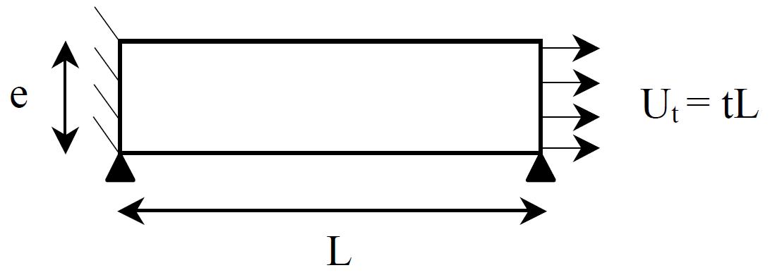
Figure 2.5-a: Representation of the bar under uniform tension
2.5.1. Analytical stability results#
We demonstrate [bib23] that there are two types of solutions to the problem studied:
The homogeneous, uniformly damaged solution.
Localized solutions that focus bar damage on a specific area.
The study of the stability of the homogeneous solution therefore amounts to verifying that the energy levels reached, considering small disturbances in the solution in the form of a location, are always greater than that obtained from the homogeneous solution.
Based on the following energy damage gradient formulation [bib24]:
\(\varphi ={\int }_{\Omega }\left(\frac{1}{2}{\left(1-\alpha \right)}^{2}{E}_{0}\epsilon {(u)}^{2}+\frac{{{\sigma }_{M}}^{2}}{{E}_{0}}\alpha +\frac{{E}_{0}{l}^{2}}{2}\nabla \alpha \mathrm{.}\nabla \alpha \right)\mathit{dx}\) eq 2.5.1‑1
the comparison of the energy levels then makes it possible to draw the stability diagram of the homogeneous solution as a function of the ratio between the length of the L bar, the internal length of the l model and the applied load*Ut* [bib23]:
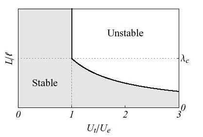
Figure 2.5.1-a: Analytical stability diagram of the member under tension
2.5.2. Stability results obtained with Code_Aster#
Using the optimization algorithm developed in the code (2.3), we find a stability diagram similar to within 5% on the load from which the instability is detected [bib25]:
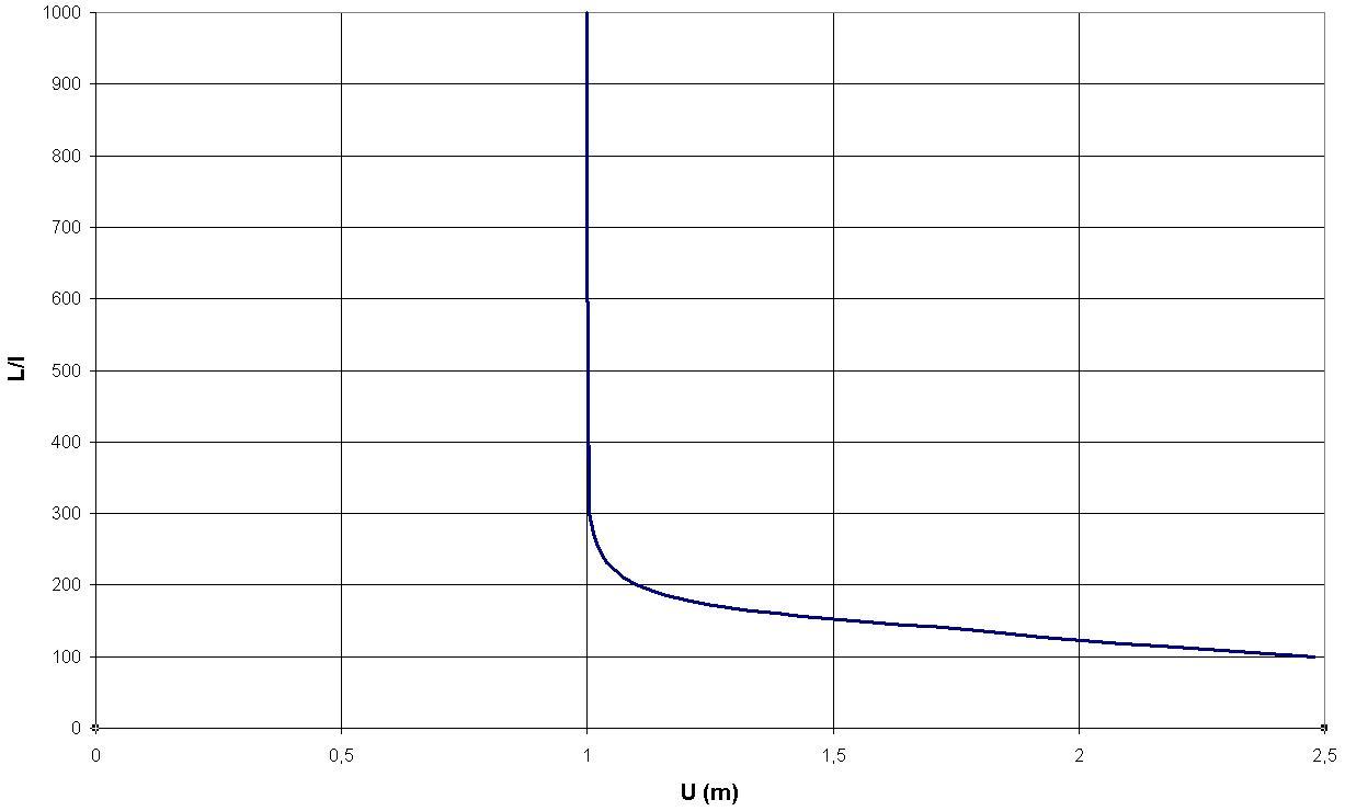
Figure 2.5.2-a: Stability diagram of the bar under tension obtained with Code_Aster
Parametric studies on the influence of the number of natural frequencies calculated and on which we rely for the stability study show that it is necessary to take about thirty for discretized problems at more or less 100,000 ddls but that it is becoming important to consider a good hundred for problems of larger size. This leads to higher CPU calculation costs, as the algorithm is time-consuming. This is why it is only really triggered when the buckling study shows that the uniqueness of the solution is no longer guaranteed.
When the algorithm shows that the stability criterion is no longer met (negative CHAR_STAB), the vector minimizing the Rayleigh quotient (eq 2.2-1) is called the instability direction. It is found as a result under the name MODE_STAB (by analogy with MODE_FLAMB for the buckling criterion). The disturbance of the current solution by this direction of instability destabilizes it and allows it to branch off towards a stable solution. In the example shown here, the direction of instability is the location of the damage on one of the two ends of the bar.
2.6. Conclusion#
Code_Aster allows stability studies to be carried out on dissipative problems such as plasticity or damage problems. The algorithm used is based on the power method to which is added the projection of degrees of freedom, in space respecting the unilateral irreversibility constraints. Its application is only really implemented when the criterion of uniqueness is violated. Otherwise, uniqueness is sufficient to guarantee stability. If the loss of stability of the solution is detected at a time step during the finite element calculation, the algorithm provides the direction to be added as a disturbance to find a stable bifurcated solution.