1. Theoretical background

1.1. Standard J-integral formulation in 2D

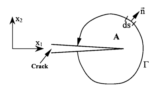
The*J* -integral [1] is widely used in fracture mechanics analyses to assess the structural integrity of industrial components. In its basic definition, the value of the*J* -integral is calculated along a small closed contour around the crack tip in a two-dimensional (2D) problem for an elastic (linear or non-linear) material subjected to a proportional monotonic stress, as shown in Figure 1. :

For a*2D* analysis, in the absence of the body forces and the crack face traction, under quasi-static conditions with a crack directed along the*x1* -axis (Figure 1), a path independent formulation of the standard*J* -integral definition is defined as ([1], [2],):

wher*Δij* is the Kronecker coefficient, schij and ui are components of stress and displacement in the Cartesian coordinates, respectively. In Equation 1, GAM*represents a curve surrounding the crack tip which begins at the lower face of the crack and ends at the upper one while*ni*represents the unit vector normal to GAM* and d*s* represents the infinitesimal path length along GAM*.

The strain energy density*W* is defined at Gauss points as:

Applying the divergence theorem, Equation 1 is transformed into a domain integral formulation as shown in [2]:

where*q* is any smoothing function defined over the area*A*, which takes the values of unity at the crack-tip node, zero on the contour GAM*, and varies from 0 to 1 within the ring of elements containing GAM*. Physically, q represents the virtual crack extension. It should be noted that the*J* -integral approach in this macro_command is equivalent to the*G-theta* method used in the operator CALC_G of*code_aster* but with a different numerical implementation. Also, q- field plays a similar role as the theta-field in CALC_G. Only the*u* and*q* fields are evaluated on nodes, and the remaining parameters are evaluated at the Gauss points.

1.2. Extension of standard J-integral 3D

Precisely planar crack surfaces, the standard*J* -integral formulation defined in Equation (1) in*2D* can be extended to a three-dimensional (3D) problem where a*2D* formulation is defined locally on each plane*Si* perpendicular to the crack front line at each crack tip point for all the points along the crack front line.

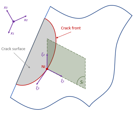
Figure 2: Definition of the local J-integral evaluation for 3D problems.

For a*3D* problem, a crack front with a global coordinate system*x1x2x3* is first defined. Then, a local coordinate system*62/23* is introduced at arbitrary crack tip point Ni of the crack front (Figure 2). The coordinate axes*04:1* and*62/2* lie in a plane*Si* normal to the crack front through Ni, kut2 is perpendicular to the crack surface, and*kut3* is tangent to the crack front. According to the basic definition of*J* -integral in*2D*, the local*J-* integral can be computed along a small outline around Ni in the*kut104:2* plane. For an arbitrary crack, the general*3D* expression of*J* -integral to perform computations in the global coordinate system*x1x2x3* can be expressed by Equation 4 at each local crack tip node Ni, as shown in [5]:

In this equation*Ac* is the area increase in the cracked surface (Figure 3) generated by the virtual crack extension*q* and*V* represents the volume (Figure 4). Details of the term*Ac* are given in Section 2.4 .In the discretised finite element space, the area increase*Ac* at the local node Ni is determined by an only moving*Ni* to*Ni* “(Figure 3). It is noted that there is no specific requirement for the shape of the volume V around the crack tip when performing this domain integral. W is the strain energy density as defined in Equation 2 and the remaining terms are the same as in Equation 3.

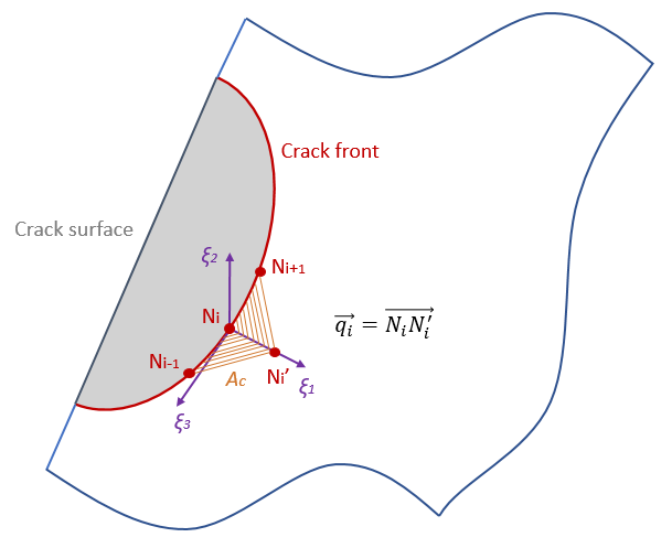
Figure 3: Definition of area increase Ac at node Ni in discretization problem.

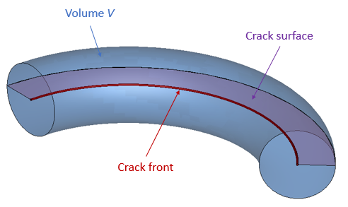
Figure 4: Definition of the volume integration V around crack front.

1.3. Modified J-integral for initial strain under proportional loads

For cases of initial strains, we define the « initial state » as the moment in time prior to the application of external loading to a cracked body. When initial strains are present, the total strain during mechanical loading*lèij* is the sum of the mechanical strain*lèmij* under load and the initial strain*lè0ij* at initial state, as shown in Equation 5:

math:

{epsilon} _ {mathit {ij}}} = {epsilon}} _ {mathit {ij}} ^ {m} + {{epsilon} _ {mathit {ij}} _ {mathit {ij}}}}} ^ {0} |} _ {mathit {initial}}mathit {state}}

It is assumed that the initial strain*è0ij* remains constant during subsequent deformation and the mechanical strain*lèmij* is related to the applied stress through the material constitutive law. Note that è0ij arises from a preliminary calculation of the initial state and more detail on the initial state is given in Section 1.1. A 3-dimensional path independent*J* -integral (Equation 6) for this loading condition can be obtained under the conditions of proportional loading as shown in [2]:

In this modified J -integral, W is defined as the mechanical strain energy density:

Note that rèmij is the sum of the elastic and inelastic strain obtained during loading of a cracked body, corrected for the inelastic strains at the initial state (Equation 11 in Section 1.5). The calculation procedure illustrated in Figure 6 of Section 1.5 shows that the initial state arises from a preliminary calculation step before the cracked body analysis (CBA) occurs. The initial strains at the initial state is effectively a constant field used in the post-processing of the results from the cracked body analysis.

1.4. Modified J-integral for initial strain under non-proportional loads

Lei [3] proposed a more general modified J -integral formulation which covers both cases with the presence of initial strains and non-proportional stress experienced during applying mechanical load (after initial state) while accounting for initial strains. Following the method of Wilson and Yu [6], Equation 4 is modified as:

with strain energy density*W* defined by Equation 7 and the total strain*œij* by Equation 5.

Practically, the*J* values obtained on the first, second, or third contours are generally dropped because of the resulting stress, strain, and displacement rate at the vicinity of the crack tip (this may depend on the mesh refinement). As a general rule of thumb, it is best practice to have a sufficiently fine mesh around the crack tip for calculations. Moreover, the correction part in the right-hand side of Equation 8 can be also affected by the potentially near tip field data, resulting in an incorrect correction to the modified J. Note that the correction part of the modified J is evaluated using the volume integration. Therefore, any errors evaluated at the near tip volume affect all the following calculations and force the path-independent modified*J* to approach an incorrect value; typically this occurs on the first or second domain. This source of error may lead to an underestimation of the modified J, and it is found that the error due to this may be significant at lower load levels (for small scale yielding conditions).

However, this error with reduces increasing load level and almost disappears when the load occurs approximately half of the yield stress-based limit. The specific reason for the error reduction at high load level is not fully identified but it is conjectured that the higher absolute*J* value at a high load level reduces the relative error [4]. In order to minimize the effect of the almost tip data on the correction term of the modified J, a very small volume surrounding the considered points on crack front is excluded from the integration volume and Equation 8 can then be modified following the method in [4]:

Here the volume*V1* is limited by two volumes*V* and*V”. The size of*V” may be determined empirically by selecting the first three contours around crack front for a reasonably finely focused mesh (see Figure 5 below). It is noted that there is no specific requirement for the shape of the volumes*V* and*V”* around the crack tip when performing this domain integral.

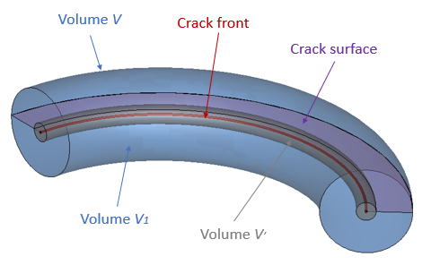
Figure 5: Definition of the volume integration domain (V1 = V - V”) around crack front.

Using Lei’s modification and in the presence of the initial strain, Equation 6 can be modified to:

1.5. Evaluation of initial strain

Numerous studies in the literature show that the values of the standard*J* -integral in Equation 4 tend to be path-independent under the presence of*residual stresses*. The path-dependence leads to the non-validity of*J* -integral as a useful constant fracture mechanics parameter. Lei*et al.* [2] proposed the modification of Rice’s J -integral to correct the formulation to produce a path-independent*J-* integral to account for*initial strains* under proportional loads.

Note that, generally speaking, a residual stress field can arise from internal strains, which could form due to non-uniform plastic deformation, non-uniform heat expansion, or local volume changes owing to phase transformations, etc. If the internal strain field produces an additional mechanical strain field (without external loading) residual stresses occur in the body. It is these such residual stress problems that can be considered as initial strain problems [2]. For this reason, only the initial strain state is treated in the modified J -integral calculation illustrated in Figure 6.

Figure 6 shows an example process to evaluate the initial strains at the « initial state. » The first step may be a preliminary non-linear analysis of the problem to generate a residual stress field in the body, which features an associated initial strain field. A user would then, in the second step, perform a CBA under loading that includes the effects of the residual stresses in the initial state. The modified J-integral computation would then occur in the third step, as a post-processing operation on the results output from the second step, using the initial strain field at the initial state evaluated in step 1.

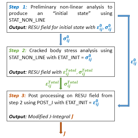
Figure 6- Example of the sequence of calculations that produce: the initial state, the CBA with initial state, modified J-integral calculation on the CBA. Example based on computations done within code_aster.

From the user’s viewpoint, it is emphasized that only the initial strain state is required as an input, and not a distinction as to the type of strain. However, the user must be aware that they need to carefully assign the initial strain state depending on the specific engineering problems to be assessed. For example, thermal loading cases allow the initial strains to be evaluated directly, but more generally, the initial strains can be determined from the total and elastic strains at the initial state (Step 1).

math:

{epsilon} _ {mathit {ij}}} ^ {ij}}} ^ {0} = {left ({epsilon}} _ {mathit {ij}}} ^ {mathit {Total}}} - {epsilon}} - {epsilon}} _ {mathit {j}}}} ^ {e}right) |} _ {mathit {initial}}mathit {Total}}} - {epsilon}} - {epsilon}} - {epsilon}} - {epsilon}} _ {epsilon}} _ {mathit {state}}} = {epsilon} _ {mathit {ij}}} ^ {p} |} _ {mathit {initial}mathit {state}}} (11)

From the developer viewpoint, it is necessary to be aware that the CBA in step 2 generates total strains which include the effect of the initial strain field, as shown by Equation

\({{\epsilon }_{\mathit{ij}}^{\mathit{Total}}={\epsilon }_{\mathit{ij}}^{e}+{\epsilon }_{\mathit{ij}}^{p}+\epsilon }_{\mathit{ij}}^{0}\)

Therefore, when evaluating*rèmij* (Equation 7) required for modified J-Integral calculations in step 3, it may be necessary to separate the initial strain from the total mechanical strain arising from the CBA in step 2. For this reason, the concept « initial state » was introduced earlier. All plastic strains before the initial state must be treated as initial strains in the post-processing calculation of step 3. Elastic strains, at the initial state, however, are recoverable and therefore contribute to the mechanical strain during step 2. The mechanical strain (Equation 7) from the CBA in step 2 is then decomposed as:

math:

{epsilon} _ {mathit {ij}}} ^ {ij}}} ^ {ij}} ^ {mathit {Total}} - {epsilon} _ {epsilon} _ {mathit {ij}} _ {mathit {ij}} _ {mathit {ij}} _ {mathit {ij}} _ {mathit {ij}}} _ {mathit {ij}} _ {mathit {ij}} _ {mathit {ij}} _ {mathit {ij}} _ {mathit {ij}} _ {mathit {ij}} _ {mathit {ij}} _ {mathit {ij}} _ {mathit {ij}} _ {mathit {ij}} _ epsilon} _ {mathit {ij}}} ^ {p}right) - {epsilon} _ {mathit {ij}} ^ {mathit {plas}} |} |} _ {mathit {initial}mathit {initial}mathit {initial}mathit {initial}mathit {initial}mathit {initial}mathit {state}} (12)

wher*lèeij* and*lèpij* are the total elastic and plastic strains, respectively, and*lèpij* | initial state is the plastic strain at the initial state, which is detailed by Lei in [2].

Furthermore, normally only the total strain energy density*Wtotal* is available in finite element software, which is not equal to*W* in Equation 7 since the plastic strains will include plastic strain accumulated before the initial state. Therefore, W must be obtained from the adjusted WTotal as:

Wher*Wp* | initial state is the plastic work done during the initial state.