3. Algorithm of POST_JMOD J-integral in code_aster#
3.1. Approach to Compute Fracture Mechanics Parameters in Presence of Initial Strain#
There are three main steps in the computation of fracture mechanics parameters in the presence of initial state:
Create a field at the initial state
There are two types of initial state: the first is a result field from a computation step (as described in section 1.5) and the second ay result from importing an external residual stress/strain field.. It is important to verify that the initial state is in auto-equilibrium. For example, from an initial stress field, one can deduce an equivalent initial stress field. By performing a dummy step with no applied loads, one can verify if the initial state is in auto-equilibrium. The user must be aware that the fields given to POST_JMOD are appropriate.
Perform a mechanics computation including initial state for a cracked structure
Post-processing using POST_JMOD
STEP 1: Create an initial state Using STAT_NON_LINE or by CREA_CHAMP If using CREA_CHAMP, verify that the initial stress is in auto-equilibrium |
||
STEP 2: Mechanical calculation with initial stress and cracked structure |
||
SIG_0 497 0+ CRACK |
→ (STAT_NON_LINE) → |
SIG 497, EPS, 0 |
STEP 3: J calculation in presence of initial state |
||
POST_JMOD =(… ETAT_INIT =_F (EPSI = EPS_0) |
||
Figure 7- Steps in computation of fracture mechanics
3.2. Steps in strategy implementation#
POST_JMOD is developed as a python based macro command in order to execute step 3 of Figure 7. The programmed algorithm is contained within POST_JMOD_ops .py. The script contains all the necessary functions in order to perform the calculation described within Section 2. However, some minor changes to the FOTRAN90 code were made in order to enable computation for large numbers of contours. This is a simple change to the size of the number of nodes defined by INFNORM_NOEU2 within defi_fond_fiss.
The general sequence of computation is described by the following diagram:
Firstly, using in built operators, the mesh geometric data, model is extracted and the field results containing the global displacement field at node points and stress, strain, energy fields at gauss points. This represents the raw information used to set up the algorithm and computation. An example of the syntax used is given:
MAIL = self.getModel () .getMesh ()
MODE = self.getModel ()
RESULTAT =__ RESU,
CONTRAINTE =( “SIGM_ELGA”),
DEFORMATION =( “EPSI_ELGA”),
ENERGIE =( “ETOT_ELGA”),)
Secondly, from the data structure of the crack defined by DEFI_FOND_FISS, information regarding the crack is extracted: element type, the presence of symmetry, opened/closed crack type, crack surfaces. This information is used to determine the number of nodes on the crack front, set of nodes on the crack surfaces through nodes of crack front. The information is also used to create logic gates within the POST_JMOD_ops .py files in order to correctly apply the computation as data structures are different sizes and types.
elemType = FOND_FISS .getCrackTipCellsType ()
ir, ib, symmeType = aster.tell me (“SYME”, FOND_FISS .getName (), “FOND_FISS”, “F”)
NP, TPFISS, ClosedCrack = no_fond_fiss (self, FOND_FISS)
Then, the virtual crack extension field is computed. This field is substitute as the*q*field in the*J -integral computation. Further details of this step are given in Section 2.1
Next, the volume domain*V*for the calculation is identified according to a user specified number of contours. Once the integral volume is determined, all nodes are extracted from this volume and the*q fields are assigned to these nodes. In this development, the number of contours must be greater than or equal to 2. Details of this step are given in Section 2.2 and 2.3.
Then, the virtual area increase of the cracked surface generated by application of virtual crack extension is calculated. To do this, the nodes on the crack surface are translated according to the virtual crack extension vectors to compute the area. Note that this is only performed to calculate the area increase and the mesh remains unchanged for the J-Integral computation. Further details of this step are given in Section 2.4.
Next, following the problem as linear/non-linear problem, the*J-integral is calculated at each instant of calculation and at each node of crack front. The calculated fields such as virtual crack extension*q*, stress, strain, strain, displacement, energy, and their gradients/divergence can be extracted from the results or can be computed using CREA_CHAMP, CREA_RESU, and CALC_CHAMP operators. The non-conventional terms are detailed in Section 2.5 and Section 2.6.
Here is a pseudo-code for the loops on moments and on nodes and the calculation/combination of terms:
Q_ FIELD
for INST in LIST_INST:
STRESS_FIELD
DISPLACEMENT_FIELD
GRAD_OF_DISPLACEMENT_FIELD
STRAIN_FIELD
GRAD_OF_STRAIN_FIELD
if presence_of_initial_strain:
INITIAL_STRAIN_FIELD
GRAD_OF_INITIAL_STRAIN_FIELD
STRAIN_ENERGY_FIELD
GRAD_OF_STRAIN_ENERGY_FIELD
for INODE in LIST_NODE:
GRAD_OF_Q_FIELD
COMPUTE EACH TERME OF EQUATIONS Error: Reference source not found AND Error: Reference source not found IN SECTION 2
J= COMBINATION OF TERMES
At the end of POST_JMOD macro_command, the results of*J*are printed under format table of*code_aster using CREA_TABLE and CALC_TABLE.
3.3. Restrictions on Element Types and Loads#
The*J* -integral may be applied to a*3D* problem where it is defined locally around the crack tip points along the crack front in the planes perpendicular to the crack front (see Figure 2), as discussed in section 1. The procedure to calculate*J* has only been developed with hexahedral elements in mind. However, for complex 3D cracks, it is possible to use the prism elements for the first ring around the crack front. It must be noted that one of the quadrangle surfaces of these prism elements should be located on one of the crack surfaces (Figure 8). This restriction comes from the difficulty in determining of crack propagation direction and of the area increase of the cracked surface with irregular meshes. The user must take to ensure an appropriate mesh is used in the computation.
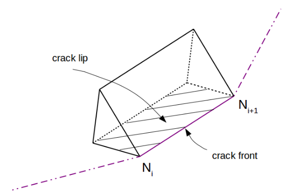
Figure 8: Definition of the pentahedral element for J calculation.
It should be emphasized that the same limit was observed in the*J* -integral development of Abaqus software [7]: « The contour integral evaluation capability of ABAQUS assumes that the elements that lie within the domain used for the calculations are quadrilaterals in two-dimensional or shell models or bricks in continuum three-dimensional models. Triangles, tetrahedrals, or wedges should not be used in the mesh that is included in the contour integral regions ».
In*code_aster*, it is possible to calculate the*J* -integral using the command POST_JMOD [U4.82.41]. The virtual crack extension field of the crack*q* is calculated automatically in this command from the information provided by the user. The current development is valid for the*3D* modeling and deals with the following conditions only:
both elastic and plastic behaviors of materials;
proportional, non-proportional and mixed mode loads;
initial strains (representing residual stress fields)
It cannot deal with cases where there is pressure on the crack surfaces.
3.4. Required existing code_aster concepts#
For the calculation of the energy release rate, it is necessary to experiment with the meshed crack via the concept of the FOND_FISS type with the command DEFI_FOND_FISS [U4.82.01]. The current version of POST_JMOD has not been yet available for non-meshed (X- FEM) crack. As discussed later, hexahedral elements need to be used in the regions around the crack tip which are used to compute domain integral.