4. Developments specific to POST_JMOD formulation#
4.1. Computation of Virtual Crack Extension Field Q#
In this section, we show how to determine the virtual crack extension field*q* which is defined by Equation 3 at each node point of crack front when the crack front is defined by straight segments and the crack surface is defined by straight segments and the crack surface is defined by flat element faces. The vector q is defined here on all the nodes within volume integration limited by number of contours and not on a line, and*q=0* for all nodes on boundary. Then, the integral is evaluated on this volume. In this development, the q value calculated by Equation 30 is used for assigning (this is not case that was done in*2D* by Lei).
We consider a crack crack crack with crack front on which the node Ni and its neighbors Ni-1, Ni+1 are presented and its surface (Figure 9). We will determine**qi* at node Ni.
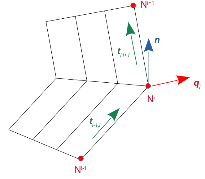
Figure 9: A crack with crack front and its surface. |
First, two vectors **ti-1, i* and **ti, i+1* along two neighboring segments of the crack front are determined:
where **ui-1*, **ui*, **ui+1* are coordinates of Ni-1, Ni, Ni+1, respectively, and ||.|| denotes vector length.
The virtual crack extension **qi* at the crack front node Ni is obtained by averaging the following two vectors:
Where n is a normalized vector of crack surface at Node Ni and can be determined as:
Finally, the virtual crack extension*q* is calculated as:
4.2. Extension of contour domain identification from 2D to 3D#
In this section, the methods to identify the domain integral in*2D* and*3D* are discussed.
For a*2D* meshed crack, an example of two contours around crack tip N are shown in Figure 10. As shown in the figure, the contours are made to coincide with the edges of the elements, the q fields are assigned on the nodes of these contours and the J-integral is evaluated on the 2D surface area enclosed by each contour.
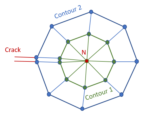
Figure 10: The defined contours around crack tip in 2D problem.
In*3D* problems, in order to illustrate the extension, we first assume that for each node along the crack front, there exists a plane perpendicular to the crack front through this node (Figure 11), e.g. plane (Pi) through node Ni. On each plane, the outline is identified in the same manner as the*2D* case for two successive planes as shown in Figure 12. These nodes become the two surfaces of the torus along the Nini+1 direction. The contours are made of the surfaces of the elements, the*q* fields are assigned on the nodes of these contours and the integral is evaluated on the*3D* volume.
As mentioned in Section 1.3, in 3*D*, hexahedral meshes are used in the contour integral regions and it is possible to use the pentahedral elements for the first ring around the crack front. This allows the existence of a plane that passes each node of crack front.
When considering the discretised problem by the finite element method, we note that it is possible that the set of nodes defining the contours that for each nodal position along the crack front may not all lie on a single mathematical plane, as the assumed theory of*J* -integrals in*3D* discussed earlier. However, they are well defined on a single surface. Note that a surface here is defined as a group of element surfaces and they do not necessarily all lie on a plane. More specifically, the left hand image in Figure 13 shows the set of nodes through node Ni where all nodes lie on a plane perpendicular to the crack front. Likewise, the right hand image of Figure 13 shows the case where the nodes may lie out of plane.
N.B. In the algorithm, no specific shape of domain is required, but it is reiterated that the user must take care in the definition of the mesh to ensure the mesh regularity coincides with the theory.
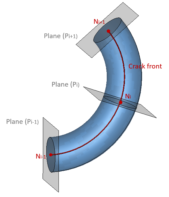
Figure 11: The local plane defined on each node of crack front in 3D.
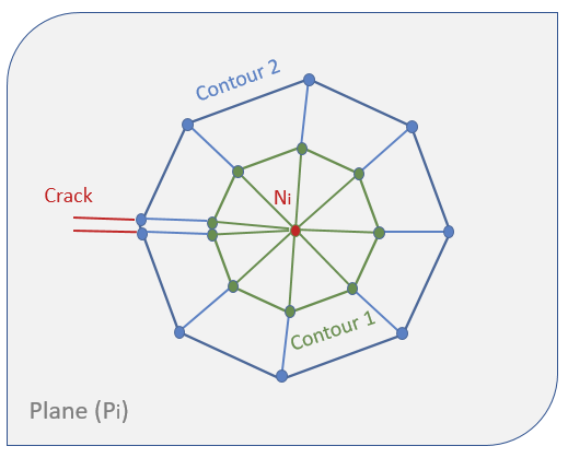
Figure 12: Definition of contour on the local plane (Pi) through the node (Ni) on crack front.
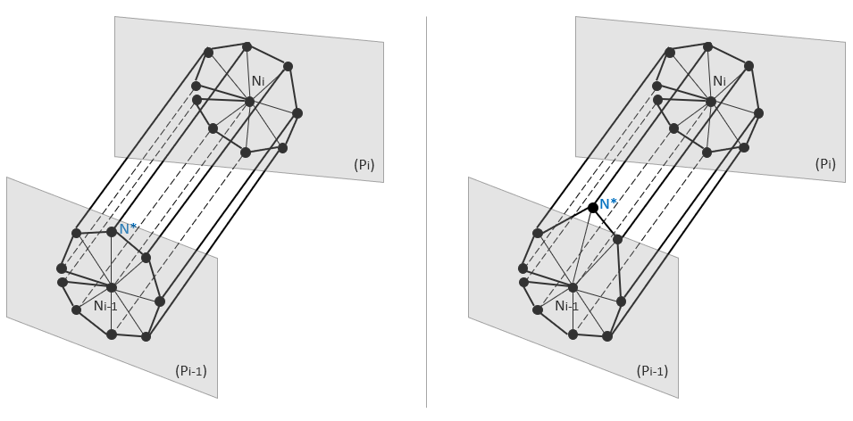
Figure 13: The defined outline on each plane in discretized problem: (left) N*node is in plane and (right) N* node is out of plane.
4.3. Identifying node and element sets within the Integral domain#
To determine the elements that compose each contour domain, POST_JMOD needs only to know the set of nodes along the crack front and the number of contours evaluated.
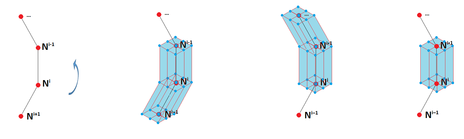
Figure 14- Domain extraction step 1. All elements with at least one node connected to the crack front are extracted for each node along the crack front. The difference in element sets between neighbouring groups is then taken.
Firstly, the nodes of the crack front are interrogated sequentially (Figure 14). This allows the creation of the sub sets of elements that have at least one node contained within each of those crack front nodes. By comparing the first element set along the crack front with its neighbouring element set, the elements contained within both sets can be extracted. These elements correspond to the elements lying on the plane emanating from each crack front nodal position.
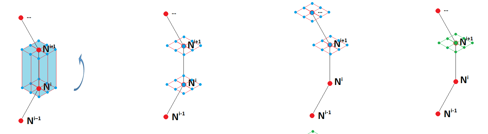
Figure 15- Domain extraction step 2. The nodes within each element set is extracted for each crack front nodal position. The neighbouring node sets are compared to obtain the intersecting nodes.
Then, the set of elements at the crack front nodal positions are interrogated sequentially (Figure 15). This allows the extraction of the node sets corresponding to the element sets. The intersection between neighbouring nodal sets is used to extract the node set attached to the first contour of elements at each crack front nodal position. These nodes correspond to the nodes lying in the plane emanating from each crack front nodal position.
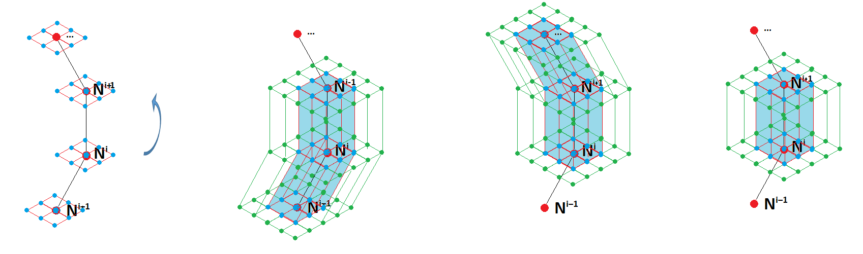
Figure 16- Domain Extraction Repeat Step 1 for Next Contour
The process is now repeated for the second contour, first allowing the extraction of elements from each crack front nodal position (Figure 16), and then allowing the extraction of node sets lying in the plane emanating from each crack front nodal position (Figure 17). The elements within the domain are used later in the POST_JMOD algorithm to perform the J computation; this is computed using with POST_ELEM command using in-built functionality to integrate over the volume (INTEGRAL). Note that only local values of J are computed along the crack front.
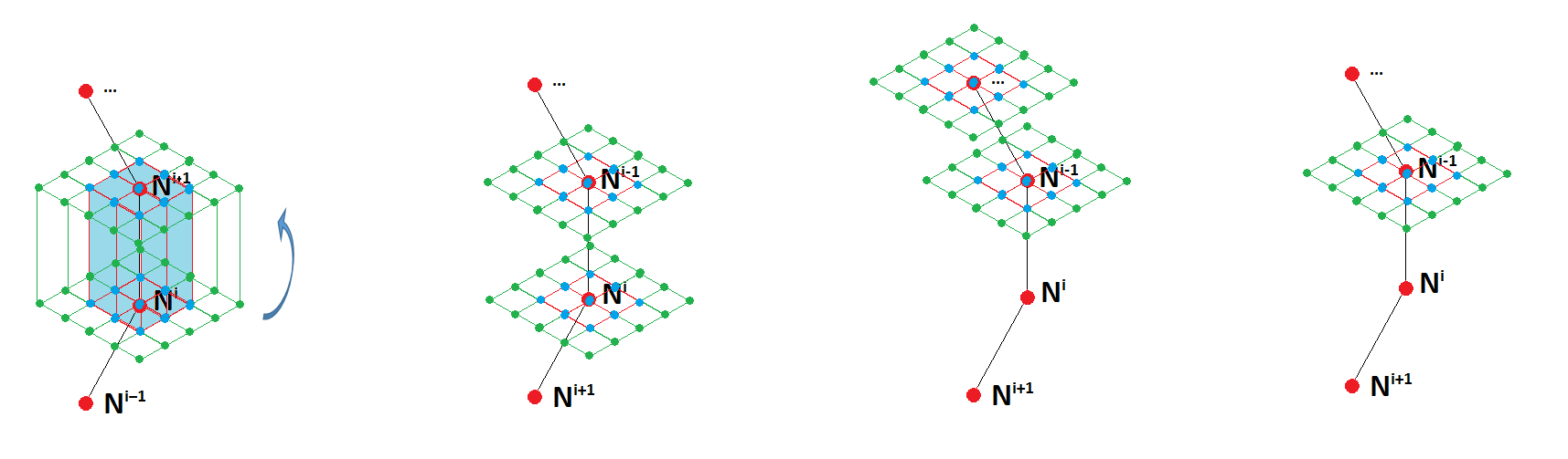
Figure 17- Domain Extraction Repeat Step 2 for Next Contour
The algorithm that does this makes use of in-built*code_aster* commands in order to define groups (or sets) of nodes and elements (DEFI_GROUP) and makes uses the specific functionality to check the difference in element sets (DIFFE) and to obtain intersections (INTERSEC). The algorithm also employs specific conditions to deal with the end most crack front nodal positions.
The domain elements and node sets are also used to assign the tags of the*q* -field. This allows the boundary nodes of each contour to be assigned a value of zero, and all other nodes within the contour to be assigned the virtual crack extension as a*q-* field.
4.4. Computation of the area increase of the cracked surface#
In a*3D* analysis, J -integral takes the increase in cracked area*Ac* due to a virtual crack extension. This increase is due to the shift of that particular node and depends on a number of considered contours. Delorenzi [5] showed an approximate formulation for a constant strain element like 8-nodes and 20-nodes 3*D* isoparametric elements but for only first contour.
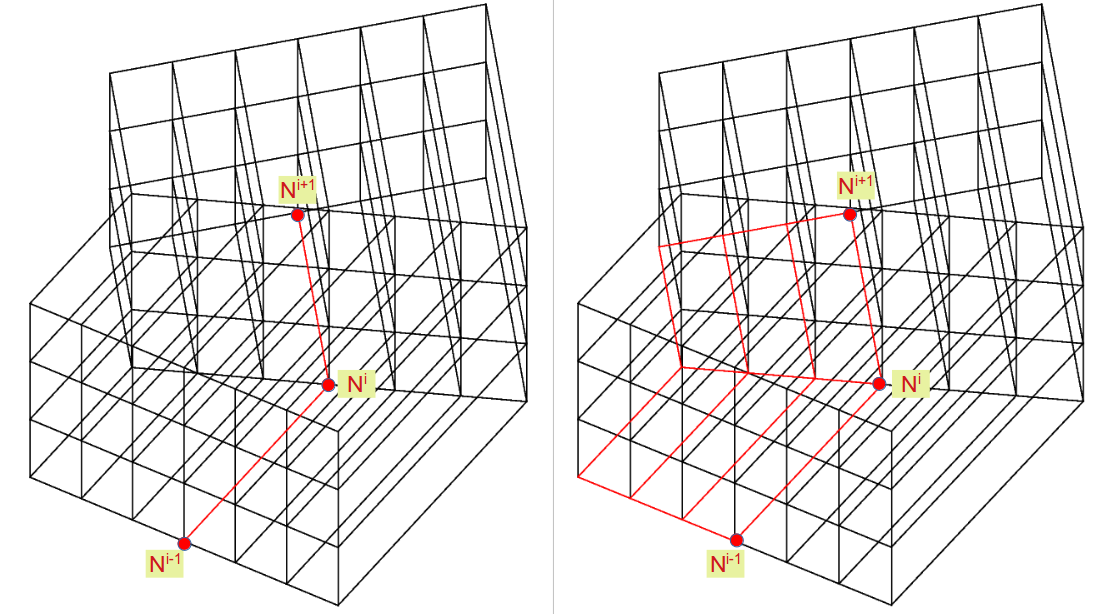
Figure 18- Crack front nodes and the crack surfaces.
We present a simple case for calculating*Ac* at node Ni on the crack front using number of contours equal to 2 to illustrate the implementation. We consider a crack with crack front on which the node Ni and its neighbors Ni-1, Ni+1 and its surfaces are presented Figure 18, and more clearly in Figure 19.
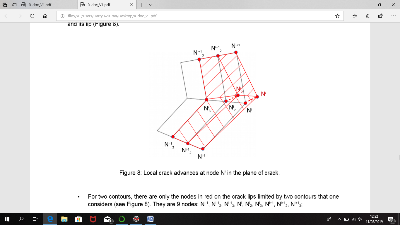
Figure 19: Local crack advances at node Ni in the plane of crack.
For two contours, there are only the nodes in red on the crack surfaces limited by two contours that one considers (see Figure 19). They are 9 nodes: Ni-1, Ni-12, Ni-12, Ni-13, Ni, Ni, Ni2, Ni3, Ni+1, Ni+12, Ni+12, Ni+13;
In the initial configuration, we calculate the initial area (in black) created by these 9 nodes:*Aini;
We only move two nodes Ni and Ni2 (in black) along vector**qi (calculated in section 2.1) to the new positions (in red). It is noted that only the nodes lie on the crack surface and within the integral domain (not boundary nodes) are affected by this movement;
Update the new surfaces (in red);
In this configuration, we calculate the new area (in red) created by these 9 nodes:*Finish;
The increase in cracked area*Ac can be calculated:
The objective of this movement is just to calculate*Ac* value and the other calculations are performed on the initial mesh. To calculate*Ac* in POST_JMOD, we use the POST_ELEM operator with INTEGRAL option by assigning a field equal to 1 on the surface which should be calculated.
4.5. Computation of gradients of deformation terms in code_aster#
In the*J* -integral formulation, we need to manipulate the gradients of the displacement, the virtual crack extension (for the standard*J*) and the strain (for the modified J with or without the initial strain, both proportional and non-proportional). The discretization of these fields are presented in Equations 15, 16 and 17. The components of these fields include:
displacement**u: *(*ux, uy, uz);
virtual crack extension**q: *(*qx, qy, qz);
strain*: (*exx, eyy, yz, ezz, exy, exz, eyz).
Because of the limit of Python to read the shape functions in*code_aster*, we use an existing principle to calculate the gradient of a field. It is noted that the strain is the results of a displacement gradient field using CALC_CHAMP operator with DEFORMATION option. It can be used when:
these fields are well determined on the nodes (TYPE_CHAM =” NOEU_XXXX_R “);
The calculation is sequentially done for each component on all components of field (3 components for**u**and**q*, and 6 components for**e.**).
For example, following steps are performed to calculate the strain gradient*lèij, k* (a non-conventional term) for the only component*èxx*:
- math:
frac {{partialepsilon} _ {mathit {ij}}} {{partial x} _ {n}}approxsum _ {k=1} ^ {mathit {ng}} ^ {ng}}sum _ {ng}}}sum _ {l=1}} ^ {3}}frac {{partial N}} _ {l}}frac {partial {eta} _ {l}} {{partial N}} {{partial N}} _ {partial {epsilon}} _ {mathit {ijk}} |} _ {mathit {NOEU}}} (32)
First, the strain field which was calculated at Gauss points by defaults is changed to that at the nodal points:
EPS_NOEU = CREA_CHAMP (TYPE_CHAM =” NOEU_EPSI_R “, OPERATION =” DISC “, MODELE = MODE, CHAM_GD = EPS_ELGA) |
The strain field EPS_NOEU has 6 components: “EPXX”, “”, “EPYY”, “”, “”, “EPZZ”, “EPXY”, “EPXZ” and “EPYZ”. We only show how to calculate the gradient of “EPXX” component as the computations for the other five components are similar.
Change the strain component “EPXX” into the displacement component “DX”:
EPS_CAL = CREA_CHAMP (OPERATION =” ASSE “, MODELE = MODE, TYPE_CHAM =” NOEU_DEPL_R “, ASSE =( _F (TOUT =” OUI “, CHAM_GD = EPS_NOEU, NOM_CMP =( “EPXX”,), NOM_CMP_RESU =( “X”,),),),),) |
Create a displacement field FIELD_CAL. Its value is (EPS_CAL, 0., 0.) with the components (“DX”, “DY”, “DZ”) respectively;
Create a result from this field:
RFIELD = CREA_RESU (OPERATION =” AFFE “, NOM_CHAM =” DEPL “, TYPE_RESU =” EVOL_ELAS “, AFFE =_F (CHAM_GD = FIELD_CAL, INST =inst),) |
Computing gradient with CALC_CHAMP with DEFORMATION option of RFIELD:
GRAD_FIELD = CALC_CHAMP (reuse= RFIELD, MODELE = MODE, CHAM_MATER = MATE, RESULTAT = RFIELD, DEFORMATION =( “EPSI_ELGA”),) GRAD_FIELD = CREA_CHAMP (TYPE_CHAM =” ELGA_EPSI_R “, OPERATION =” EXTR “, RESULTAT = GRAD_FIELD, NOM_CHAM =” EPSI_ELGA “,) |
This field GRAD_FIELD have six components (“EPXX”, “EPYY”, “”, “”, “”, “”, “EPZZ”, “EPXY”, “”, “”, “) and based on the formulation: œij = ½ (ui, j+ uj, i), we can deduce the gradient results as: EPXZ EPYZ
e*xx, x = GRAD_FIELD. EXTR_COMP (“EPXX”, [“MAIL”,], 1) ½ * e xx, y = GRAD_FIELD. EXTR_COMP (“EPXY”, [“MAIL”,], 1) ½ * e xx, z = GRAD_FIELD. EXTR_COMP (“EPXZ”, [“MAIL”,], 1) |
For a completed calculation of strain gradient*lèij, k*, we make a loop from step 1 to step 6 on all components of strain e..
4.6. Computation of Strain Energy Density Term and Its Gradient#
Computation of strain energy
Without initial strain, the strain energy W can be extracted from the results of calculation STAT_NON_LINE or MECA_STATIQUE
W = CREA_CHAMP (TYPE_CHAM =” ELGA_ENER_R “,
OPERATION =” EXTR “,
RESULTAT = RESU,
NOM_CHAM =” ETOT_ELGA “,
INST =insert,)
In presence of initial strain EPS0, the mechanical strain EPSI is first calculated, then the strain energy W is computed:
EPSI_TOT = CREA_CHAMP (TYPE_CHAM =” ELGA_EPSI_R “,
OPERATION =” EXTR “,
RESULTAT = RESU,
NOM_CHAM =” EPSI_ELGA “,
INST =insert,)
EPSI = CREA_CHAMP (TYPE_CHAM =” ELGA_EPSI_R “,
OPERATION =” ASSE “,
MODELE = MODE,
ASSE =( _F (CHAM_GD = EPSI_TOT, TOUT =” OUI “,
CUMUL =” OUI “, COEF_R =1. ),
_F (CHAM_GD = EPS0, TOUT =” OUI “,
CUMUL =” OUI “, COEF_R =-1.),),)
CHW = CREA_CHAMP (OPERATION =” ASSE “, TYPE_CHAM =” ELGA_NEUT_R”,
MODELE = MODE, PROL_ZERO =” OUI “,
ASSE =( _F (TOUT =” OUI “, CHAM_GD = EPSI,
NOM_CMP =( “EP**”,), NOM_CMP_RESU =( “X*”,),),),
_F (TOUT =” OUI “, CHAM_GD = SIGM,
NOM_CMP =( “IF**”,), NOM_CMP_RESU =( “X*”,),),),
),)
CHFMUW = FORMULE (1/2*SIGM* EPSI)
W = CREA_CHAMP (OPERATION =” EVAL “,
TYPE_CHAM =” ELGA_NEUT_R “,
CHAM_F = CHFMUW,
CHAM_PARA =( CHW,),)
Computation of gradient of strain energy
In the similar way of gradient of strain in Section 2.5, the discretization of gradient of W is defined in Equation 33 and was performed in*code_aster* as:
- math:
frac {{partialepsilon} _ {mathit {ij}}} {{partial x} _ {n}}approxsum _ {k=1} ^ {mathit {ng}} ^ {ng}}sum _ {ng}}}sum _ {l=1}} ^ {3}}frac {{partial N}} _ {l}}frac {partial {eta} _ {l}} {{partial N}} {{partial N}} _ {partial {epsilon}} _ {mathit {ijk}} |} _ {mathit {NOEU}}} (33)
Change the strain energy component calculated above into the displacement component “DX”:
W_ CAL = CREA_CHAMP (OPERATION =” ASSE “, MODELE = MODE,
TYPE_CHAM =” NOEU_DEPL_R “,
ASSE =( _F (TOUT =” OUI “,
CHAM_GD =__ WELAS_NOEU,
NOM_CMP =( “ETOT_ELGA”,)
NOM_CMP_RESU =( “X”,),),),)
Create a displacement field FIELD_CAL. Its value is (W_ CAL, 0., 0.) with the components (“DX”, “DY”, “DZ”) respectively;
Create a result from this field:
RFIELD = CREA_RESU (OPERATION =” AFFE “, NOM_CHAM =” DEPL “, TYPE_RESU =” EVOL_ELAS “, AFFE =_F (CHAM_GD = FIELD_CAL, INST =inst),) |
Computing gradient with CALC_CHAMP with DEFORMATION option of RFIELD:
GRAD_FIELD = CALC_CHAMP (reuse= RFIELD, MODELE = MODE, CHAM_MATER = MATE, RESULTAT = RFIELD, DEFORMATION =( “EPSI_ELGA”),) GRAD_FIELD = CREA_CHAMP (TYPE_CHAM =” ELGA_EPSI_R “, OPERATION =” EXTR “, RESULTAT = GRAD_FIELD, NOM_CHAM =” EPSI_ELGA “,) |
This field GRAD_FIELD have six components (“EPXX”, “EPYY”, “”, “”, “”, “”, “EPZZ”, “EPXY”, “”, “”, “) and based on the formulation: œij = ½ (ui, j+ uj, i), we can deduce the gradient results as: EPXZ EPYZ
W , x = GRAD_FIELD. EXTR_COMP (“EPXX”, [“MAIL”,], 1) ½ W, y* = GRAD_FIELD. EXTR_COMP (“EPXY”, [“MAIL”,], 1) ½ W, z* = GRAD_FIELD. EXTR_COMP (“EPXZ”, [“MAIL”,], 1) |