2. Formulation of the constitutive law#
2.1. Actual Problem and Modelling Assumptions#
We consider a concrete panel reinforced by two steel grids located on one side and the other of the middle plane of the plate. The thickness \(H\) of the plate is considered to be small compared to its overall lateral dimensions \({L}_{1}\) and \({L}_{2}\), see Figure 2‑1, and the grids are composed with a periodic pattern of natural periodicity along \({e}_{{x}_{1}}\) and \({e}_{{x}_{2}}\) directions of the same length order as \(H\). Moreover we consider that external loading and inertia forces spatial distributions are « smooth » with respect to the thickness \(H\) of the plate and restricted to the low frequency range, as usual for seismic studies. Thus, it is possible to define a Reference Volume Element (RVE), denoted hereafter by \(\Omega\), including both concrete and steel grids, whose lateral dimensions are \({l}_{1}\) and \({l}_{2}\), see Figure 2‑1. We assume that the ratio of the lateral dimensions \({l}_{1}\) or \({l}_{2}\) over the dimensions \({L}_{1}\) or \({L}_{2}\) of the whole plate is of the same length order as the ratio of the plate thickness \(H\) over its lateral dimensions.
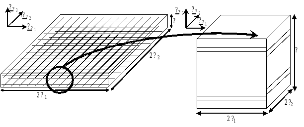
Figure 2.1-a :: ** RVE \(\Omega\) definition from the actual RC plate geometry.
We are interested in deriving an overall macroscopic plate constitutive relationship and the previous geometrical characteristics lead us to use a multi-scale analysis or a homogenization technique, as it was already proposed in the literature for many decades. In the case where components are assumed to be linear elastic, this multi-scale approach has been justified by using an asymptotic expansion method on three-dimensional elasticity equations. It leads to the well-known bi-dimensional linear Love-Kirchhoff’s thin plate theory if the dimensionless size of heterogeneities is of the same order that the relative slenderness of the solid, [bib16].
Both periodicity directions \({e}_{{x}_{1}}\) and \({e}_{{x}_{2}}\), corresponding to steel grid rebar directions, will be preferred directions for the sequel of this document. The chosen microscopic coordinate system will be the steel grid coordinate system \((O,{e}_{{x}_{1}},{e}_{{x}_{2}},{e}_{{x}_{3}})\), where \({e}_{{x}_{3}}={e}_{{X}_{3}}\) and \(O\) is the center of the considered RVE. The plane \({x}_{3}=0\) is the mid-plane of the RVE.
Upper and lower faces of the RVE are assumed to be free of charge, see [bib16].
Given the fact that material considerations for the actual RC plate problem are complex, several simplifications have been proposed. As reported in Suquet’s work (Suquet, 1993), the essential properties of the macroscopic homogenised model are directly defined from average energetic quantities that are computed from microscopic corresponding ones in the RVE and from some optimization arguments associated to local thermodynamic equilibrium — especially in the standard generalised materials context (Halphen & Nguyen, 1975). Therefore, it is believed that average quantities can catch with a reasonable good agreement the overall behaviour of an actual RC plate, even if the detail of microscopic phenomena is roughly idealized. The constitutive hypothesis about materials and their bond behaviours, needed to formulate the mathematical expression of the model are listed below with their justifications
2.1.1. Materials behaviour in RVE \(\Omega\)#
Hyp 1. Steel is considered linear elastic, without irreversible plastic strains, as we do not consider ultimate states of the RC plate. We denote by \({a}^{s}\) the corresponding elastic tensor.
Hyp 2.Concrete is considered elastic and damageable, according to the following constitutive model \(\text{}\sigma ={a}^{c}(d):\text{}\varepsilon\), \(d\) being a scalar damage variable idealising distributed cracking. The associated induced anisotropy is modelled through a suitable definition of \({a}^{c}(d)\). Concrete rigidity tensor \({a}^{c}(d)\) is defined by its initial undamaged value \({a}^{c}(0)\), whose components are reduced by a decreasing convex damage function \(\xi (d)\). We will give more details about the concrete constitutive model in section 4.2.
2.1.2. Steel-concrete interface in RVE \(\Omega\)#
Hyp 3. Concrete and steel rebar can slide one on the other beyond a given threshold.
Hyp 4. The bond status at steel-concrete interface is either sticking or sliding. Normal separation is not allowed. We do not consider any interface elastic energy associated with the sliding motion.
Hyp 5. The relative steel-concrete sliding, appearing after concrete damage and transmission of internal forces from concrete to steel rebar, can occur only in the two preferred directions \({e}_{{x}_{1}}\) and \({e}_{{x}_{2}}\) – along longitudinal rebar. It can differ whether considering the bar of the upper grid or of the lower grid, thus allowing to take into account its consequence on the RC plate flexural behaviour. Let’s denote by \({\Gamma }_{b}\) the generic steel-concrete interfaces along \({e}_{{x}_{1}}\) or \({e}_{{x}_{2}}\).
Hyp 6. Steel rebar orthogonal to the sliding direction – i.e. either perpendicular grid rebar or transversal rebar – are considered to prevent relative sliding. As a consequence, steel-concrete sliding is periodical with a period equal to the spacing between two consecutive grid bars in the considered sliding direction. This defines the lateral dimensions of the RVE \(\Omega\).
2.1.3. Non-uniform damage in RVE \(\Omega\)#
Hyp 7. In order to idealise the non-uniform damage distribution of concrete along the steel rebar, concrete domain in the RVE is in fact divided into two sub-domains associated respectively to sound concrete and damaged one. Therefore, we define a whole RVE partition into two sub-domains \({\Omega }_{\mathrm{sd}}\) and \({\Omega }_{\mathrm{dm}}\), respectively. The \({\Gamma }_{s}\) interface between these two sub-domains is assumed to be totally stuck.
Actually, concrete of the plate is not damaged in a uniform way in its volume. In order to idealize this phenomenon, one should introduce a non-uniformly distributed damage variable d in the whole RVE. Nevertheless, according to the Suquet’s work (Suquet, 1987), this non-uniformity of the microscopic internal variable field leads to the necessity to consider an infinite number of macroscopic internal variables at each macroscopic material point. This issue prevents the practical use of the macroscopic standard generalised model that would result from the chosen microscopic ones. However, still according to (Suquet, 1987), it is possible to reduce this number of internal variables to a finite one if it can be demonstrated that these internal variables are uniform or piecewise uniform or more generally described by a vector space of finite dimension. The standard generalised character of the macroscopic model is obtained from the microscopic scale behaviours thanks to the usual properties of Caratheodory’s functions of Convex Analysis. Thus, if such a chosen set of internal variables can represent the actual material state in the RVE, with a sufficient approximation degree, it is possible to build a macroscopic standard generalised model with a finite number of macroscopic internal variables. In our study, in order to restrict the number of macroscopic internal variables, we decided to define only one microscopic internal variable d for damage, considered as piecewise uniformly distributed inside the whole RVE and two sets of materials representing two different states of materials representing two different states of damage in concrete located in sub-domains \({\Omega }_{\mathrm{sd}}\) and \({\Omega }_{\mathrm{dm}}\). This distribution of microscopic damage allows in a simple way the representation of the « tension-stiffening » effect (Combescure et al., 2013). The values of microscopic and macroscopic internal variables \(d\) and \(D\) are then equated, for the sake of simplicity, without losing any generality, since the only matter is the actual value of the respective elastic stiffness tensors.
Hyp 8. In order to take into account the a priory non-uniform damage in the RVE thickness, two damage variables will be set up corresponding to the piecewise damage in the upper and lower halves of the RVE.
This leads to a macroscopic damage also decomposed into two macroscopic variables \({D}^{1}\) and \({D}^{2}\).
This strong hypothesis of microscopic damage variable stepped distribution is about to represent common experimental observations during four points bending tests on RC plates: cracks opened in tension parts of the plate appear and propagate dynamically almost instantaneously through about the half of thickness. This crack propagation time scale is much smaller than the one considered in seismic analysis and it is then adequate to separate damage into two variables depending on the position \({x}_{3}\) in the plate thickness. The distinction between those two damage steps is chosen to be at the exact middle plane \({\Gamma }_{m}\) of the plate, being the perfectly stuck interface between upper and lower halves of the RVE. This strong approximation is in accordance with reinforced concrete design standards and regulations where it is advised to consider only half of the concrete section, for bending design, e.g. (CEB - FIP Model Code 1990, 1993). In the sequel, microscopic and macroscopic damage variables will be respectively noted \({d}^{\zeta }\) and \({D}^{\zeta }\) depending on if the considered variable is the one of the upper (\(\zeta =1\)) or lower (\(\zeta =2\)) half of the RVE, see.
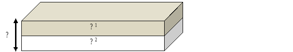

Figure 2.1.3-a :: ** Depiction of the microscopic damage variable \(d\) discretised in the RVE thickness.
Once admitted this distinction between upper and lower halves of the RVE, sub-domains \({\Omega }_{i}\) (\(i=\mathrm{sd},\mathrm{dm}\), according to the damage status) and steel-concrete interfaces \({\Gamma }_{b}\) must be split respectively in \({\Omega }_{i}^{1}\), \({\Omega }_{i}^{2}\) and \({\Gamma }_{b}^{1}\), \({\Gamma }_{b}^{2}\). Interfaces \({\Gamma }_{b}^{1}\) and \({\Gamma }_{b}^{2}\) will then be denoted by \({\Gamma }_{b}^{\zeta }\), with \(\zeta =\mathrm{1,2}\).
2.1.4. Non-uniform steel-concrete debonding in RVE \(\Omega\)#
Let’s consider, in the RVE sketched at, that sliding can occur at steel-concrete interfaces \({\Gamma }_{b}^{\zeta }\) along the \({e}_{{x}_{1}}\) or \({e}_{{x}_{2}}\) directions.
The shapes of sliding functions \({\eta }^{\zeta }(x)\) at the interfaces \({\Gamma }_{b}^{\zeta }\) should result from the mechanical energy minimization and then depends on the loading history in the RVE. Thus, they remain unknown before the introduction of macroscopic loading over the whole plate and cannot be determined a priori. As a consequence, the choice is made to prescribe*a priori* shapes for these functions in order to process conveniently to the periodic homogenization with a limited number of variables. Moreover, as well as damage has been chosen piecewise uniform inside the whole unit cell, it appears necessary to define sliding along each rebar from one only parameter per direction and per grid. Several possibilities can then be chosen: either the tangential displacement gap corresponding to the sliding is constant, or bond-stress induced by this sliding are. According to (Marti et al. 1998), debonding induced stress are assumed to be piecewise constant.
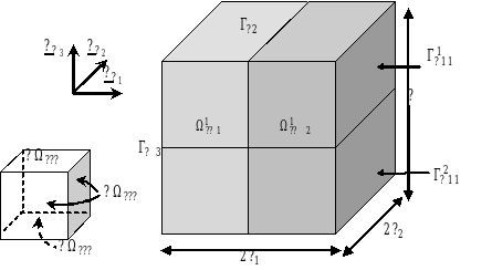
Figure 2.1.4-a :: ** Depiction of the sub-domains within the RVE thickness.
Hyp 9 .Considering the previous observation from (Marti et al 1998), a bilinear sliding function (sketched at) is chosen — corresponding to piecewise bond stresses at the interface \({\Gamma }_{b}^{\zeta }\). This sliding function is only parameterised by its amplitude, its periodicity being fixed by the one of the RVE.
Hyp 10. Moreover, it will be considered that steel-concrete sliding vector in the \(e({x}_{\alpha })\) direction, denoted by \({\eta }_{\alpha }^{\zeta }\), depends only on the coordinate \({x}_{\alpha }\): it takes the same value at any point located at the steel-concrete interface \({\Gamma }_{b}^{\zeta }\) for a given \({x}_{\alpha }\). Let’s denote by \({\stackrel{ˆ}{\eta }}_{\alpha }^{\zeta }({x}_{\alpha })\) the sliding function of unitary amplitude for the \(e({x}_{\alpha })\) direction. As a result: \({\stackrel{ˆ}{\eta }}_{\alpha }^{\zeta }({x}_{\alpha })={E}_{\alpha }^{\eta \zeta }\mathrm{.}{\stackrel{ˆ}{\eta }}_{\alpha }^{\zeta }({x}_{\alpha })\mathrm{.}e({x}_{\alpha })\), \({E}_{\alpha }^{\eta \zeta }\) being its amplitude. Moreover, we observe that \(\frac{1}{{l}_{\alpha }}{\int }_{-{l}_{\alpha }}^{{l}_{\alpha }}{\stackrel{ˆ}{\eta }}_{\alpha }^{\zeta }{\mathrm{dx}}_{\alpha }=1\).
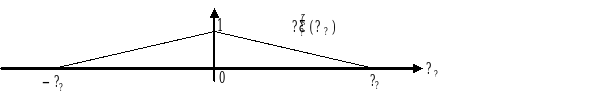
Figure2.1.4-b: Periodic sliding shape function distribution \({\stackrel{ˆ}{\eta }}_{\alpha }\) along the \(e({x}_{\alpha })\) direction with unitary amplitude in the RVE.
2.1.5. Overall strains measures and macroscopic state variables on RVE \(\Omega\)#
Now, according to the previous selection of phenomena to be idealized, we have to define a set of independent state variables, able to describe the mechanical state evolutions of the RC plate structural element at the macro-scale. First of all, the local microscopic displacement field \(u\) in the RVE \(\Omega =\text{}\cup {\Omega }_{i}^{\zeta }\) (\(i=\mathrm{sd},\mathrm{dm}\) in concrete, and \(i=s\) in steel rebar) is split into a regular part \({u}^{r}\) and a discontinuous one \({u}^{d}\), associated with the debonding relative displacement defined by the debonding relative displacement defined by the \({\eta }_{\alpha }^{\zeta }\) functions (Hyp 10) at the steel—concrete interfaces \({\Gamma }_{b}^{\zeta }\).
The overall strains measures defined as the result of the homogenization of thin plate are the following mean surface strain tensors of second order, according to Kirchhoff-Love’s kinematics (Caillery & Nedelec, 1984): macroscopic membrane strain tensor \(E\), whose components are denoted by, and whose components are denoted by \({E}_{\mathrm{\alpha \beta }}\), and macroscopic bending strain tensor \(K\) (curvature at first order), whose components are denoted by \({K}_{\mathrm{\alpha \beta }}\). As we denote by \(\varepsilon (u)\) the microscopic strain tensor associated to local displacement field \(u\) in the RVE \(\Omega =\text{}\cup {\Omega }_{i}^{\zeta }\), the components of \(E\) and \(K\) tensors are defined by the following average linear operators from the regular part \({u}^{r}\) of the displacement field:
In the sequel, the following notation \(\text{<}\cdot {\text{>}}_{\Omega }=\frac{1}{\mid \Omega \mid }{\int }_{\text{}\cup {\Omega }_{i}^{\zeta }}\cdot \mathrm{dV}\) stands for the average value of the considered field in the RVE. We can easily observe that the expressions in (2 1-2) encompass the usual definition for homogeneous plate kinematics.
We must now deal with the non-regular part \({u}^{d}\) of the displacement field in the RVE. In the sequel \(〚\mathrm{.}〛\) stands for the jump operator on the steel-concrete interface. So, we define the macroscopic sliding strain tensor \({E}^{\mathrm{\eta \zeta }}\) as the average of sliding on each steel-concrete interface \({\Gamma }_{b}^{\zeta }\). First, we observe that the contribution of discontinuous displacement \({u}^{d}\) to the macroscopic strain tensors vanishes, due to Hyp 4 and Hyp 10 (Andrieux et al., 1986):
Where \(n\) is the outward normal at the steel-concrete interface \({\Gamma }_{b}^{\zeta }\) and \(\text{}\otimes {\text{}}^{s}\) stands for the symmetrised dyadic tensor product. According to Hyp 4, the displacement discontinuity \(〚{u}^{d}〛={\eta }^{\zeta }(x)\) at the interface \({\Gamma }_{b}^{\zeta }\) does not include any opening or separation in the \(n\) direction, but only tangential sliding \({\eta }_{\alpha }^{\zeta }\). Extending the proposed definition by (Combescure et al., 2013), the components of \({E}^{\mathrm{\eta \zeta }}\) are:
Indeed, the only non-zero components of tensor \({E}^{\mathrm{\eta \zeta }}\) are \({E}_{\mathrm{\alpha \alpha }}^{\mathrm{\eta \zeta }}\). Vector \({E}^{\mathrm{\eta \zeta }}\) will then more conveniently be considered in the following as a first-order tensor of the plate mean surface, whose components are denoted by \({E}_{\alpha }^{\mathrm{\eta \zeta }}\).
The macroscopic primal state variables associated with the DHRC proposed model are then: membrane strains \(E\) and bending strains \(K\) tensors, damage variables \({D}^{\zeta }\) on upper and lower halves of the homogenised plate, sliding strain \({E}^{\mathrm{\eta \zeta }}\) vectors on upper and lower grids. These variables will be used to define state functions, as the macroscopic free energy density \(W(E,K,{D}^{\zeta },{E}^{\eta \zeta })\).