4. Finite Element implementation#
The non-linear DHRC constitutive model formulated for plate structural element has been implemented for a DKT - CST plate finite element family (Batoz, 1982), see [R3.07.03], allowing a rather efficient and versatile modelling of complex building geometries. We note that the curvature tensor \(K\) has opposite components in the notations used by the notations used by plates elements in*Code_Aster*, see [R3.07.03]: the sub-matrices \({A}^{\mathrm{mf}}\) and \({B}^{f\zeta }\) have to be multiplied by \(-1\).
The numerical integration of DHRC constitutive model lies on direct implicit time discretization method (Nguyen, 1977), (Simo & Taylor, 1985), which is included in the Newton” method with an elastic predictor step followed by a « plastic » corrector step, at the global balance equations stage.
At the beginning of each time step, trial generalised stresses are calculated by achieving a fully elastic response rate, with an elastic tensor evaluated for the previous damaged state. In what follows, the superscript \({\left\{\mathrm{.}\right\}}^{\text{+}}\) associated to the unknown variables of the problem refers to the converged state at the end of the local integration, whereas the superscript \({\left\{\mathrm{.}\right\}}^{\text{-}}\) refers to the previous converged state. It is useful to differentiate activated and non-activated macroscopic mechanisms among the six possible ones — two evolving damage \({D}^{\rho }\) variables, four evolving debonding \({E}^{\mathrm{\eta \rho }}\) components — to avoid unnecessary computation. Therefore, at each Gauss point, we get back for initialising:
: label: eq-4
(begin {array} {} {D} ^ {{rho} ^ {rho} ^ {{(1)}}}\ {E} ^ {(1)}}end {array}) = (begin {array}) = (begin {array} {} {}})) = (begin {array}})) = (begin {array})) = (begin {array} {})) = (begin {array} {})) = (begin {array} {})) = (begin {array} {})) = (begin {array} {})) = (begin {array} {})) = (begin {array} {})) = (begin {array} {})) = (begin {array} {}))} ^ {(text {-})}}}end {array})
Then, the new internal variables are computed via a local implicit resolution of non-linear equations (flow rules) based on Newton’s method, at the \({k}^{\mathrm{th}}\) iteration:
: label: eq-4
(begin {array} {} {D} ^ {{rho} ^ {rho} ^ {(k+1)}}}\ {underline {E}}} ^ {etazeta} ^ {(k+1)}}}end {array}}}}end {array}}}end {array})}}end {array})}}end {array})) = (begin {array})) = (begin {array} {} {{array})) = (begin {array} {} {D}} ^ {rho} ^ {rho}} ^ {etazeta} ^ {(k+1)}} ^ {(k+1)}} {(k+1)}}}\ {underline {E}} ^ {{etazeta} ^ {(k)}}}end {array}) - {(J)} ^ {(k)}mathrm {.} (begin {array} {} {f} _ {{d} _ {{d} ^ {rho}}} ({G} ^ {rho}})\ {f} _ {{eta} ^ {eta} ^ {pi}} ^ {pi}}} ^ {pi}}} ^ {pi}}} ^ {pi}}} ^ {pi}}} ^ {pi}}} ^ {pi}}} ^ {pi}}} ^ {pi}}} ^ {pi}}} ^ {pi}}} ^ {pi}}} ^ {pi}}} ^ {pi}}} ^ {pi}}} ^ {pi}}} ^ {pi}}} ^ {pi}}} ^ {})
The Jacobian matrix \(J\) of all activated macroscopic threshold functions (3.2-23) is computed by means of the closed-form expression established hereafter if all six thresholds are activated:
: label: eq-4
{J} _ {6times 6} =(begin {array} {{2}} {cc}frac {-1} {{G} ^ {mathrm {crit}}}} (frac {{partial} ^ {2} W} W} {partial {2} W}} {partial {D}} ^ {zeta}}} (frac {{partial} ^ {2} W} {partial} W} {partial {2} W} {partial {D} ^ {D} ^ {D} ^ {zeta}}) &frac {-1} {{G}} ^ {2} W} {partial {2} W} {partial {2} W} {partial {D} ^ {D} ^ {zeta}}mathrm {write}}} (frac {partial {B}} ^ {zeta} (D)} {partial {D} ^ {zeta}}: (begin {array} {} {} E\ Kend {array}) +frac {partial {B} ^ {partial C} {zeta}} {zeta}} {E} ^ {etazeta}} {E} ^ {etazeta}})\frac {-2 {Sigma} ^ {Sigma} ^ {eta}} {{eta}} {{({Sigma}} ^ {2}})} ^ {partial {B}} ^ {zeta} ^ {zeta} (D)} {zeta}}} {partial {D}} ^ {zeta}}): (begin {array} {}} (frac {partial {B}} ^ {partial {B}} ^ {zeta}} ^ {zeta}}): (begin {array} {}} (frac {partial {B}} ^ {partial {B}} ^ {zeta}} ^ {zeta}}): (begin {array} {}} +frac {partial C} {partial {D} ^ {zeta}} {zeta}} {E} ^ {etazeta}) &frac {-2} {{({Sigma}} ^ {sigma} ^ {sigma} ^ {sigma} ^ {sigma} ^ {sigma} ^ {sigma} ^ {sigma} ^ {sigma} ^ {sigma} ^ {sigma} ^ {sigma} ^ {sigma} ^ {sigma} ^ {sigma} ^ {sigma} ^ { (C (D)mathrm {.} {Sigma} ^ {eta})end {array})
We recall, see (3.2-2), that:
: label: eq-4
2frac {{partial} ^ {2} W} {partial {D}} {partial {D} ^ {zeta}} = (begin {array} {} E\ Kend {array}):frac {partial {D}} {partial} ^ {2} A (D)} {partial {D} ^ {rho} {rho}{partial} end {array}):frac {{partial} {array}):frac {{partial} {array}):frac {partial} ^ {partial} ^ {2} A (D)} {partial {D} ^ {rho} {rho}{partial} end {array}):frac {{partial} {array})zeta}}: (begin {array} {} {} E\ Kend {array}) +2 (begin {array} {} E\ Kend {array}):frac {{partial} ^ {2} ^ {2} B (2}} B (D)}} {partial {D}}mathrm {.}} {E} ^ {eta} + {E} ^ {eta}mathrm {.} frac {{partial} ^ {2} C (D)} {partial {D} ^ {rho}partial {D} ^ {zeta}}}mathrm {.} {E} ^ {eta}
This matrix is diagonal, by construction of the tensors \(A(D)\), \(B(D)\), \(C(D)\).
The estimated new state is so corrected to satisfy the discretised forms of the thresholds of damage and debonding, until a prescribed tolerance is reached on each threshold. The overview of the implicit integration algorithm is drawn at. in a first step, the activated thresholds are determined. Then the rates of the corresponding internal variables are solved by the Newton’s method. The all six thresholds are verified, and if some other ones are reached, the non-linear system is updated. At the end, all the local variables are updated.
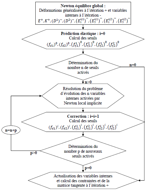
Figure 4-a : Chart of the constitutive law implicit integration.
Once the calculation of the new internal variables is done, we perform the new stress resultants, see (3.2-11) and (3.2-12); finally one calculates the tangent stiffness operator from the first variations of \(E\) and \(K\) and and corresponding first variations of \(D\) and \({E}^{\eta \zeta }\):
: label: eq-4
begin {array} {} (begin {array} {} {}frac {dN} {dE}frac {dM} {dE}end {array}begin {array} {}frac {dN} {dK} {dK}\ frac {dK} {dK} {dK}end {array}}end {array} {} {A} {} ^ {mathrm {mm}}} (D)\ {A} ^ {mathrm {fm}} (D)end {array}}begin {array} {} {A} ^ {mathrm {mf}} (D)\ {A}} ^ {mathrm {fm}} ^ {mathrm {fm}} ^ {ff}}} (D)end {array}} {A}}} (D)\ {A}}} (D)\ {A}} (D)\ {A}} (D)\ {A}} (D)\ {A}} (D)\ {A}} (D)\ {A}} (D)\ {A}} ^ {A}} ^ {A} ^ {A} ^ {A} ^ {A} ^ m {mm}} (D)mathrm {.} E+ {A} _ {, D} ^ {mathrm {mf}} (D)mathrm {.} K\ {A} _ {, D} {, D} {, D}} ^ {, D} ^ {mathrm {fm}}} (D) ^ {mathrm {fm}}} (D)mathrm {fm}} (D)mathrm {fm}} (D)mathrm {fm}} (D)mathrm {fm}} (D)mathrm {fm}} (D)mathrm {fm}} (D)mathrm {fm}} (D)mathrm {fm}} (D)mathrm {} (D)mathrm {.} Kend {array})otimes (begin {array} {}frac {partial D} {partial E}\ frac {partial D} {partial D} {partial D} {partial K} {partial K}\ partial K}\ partial K}\ partial K}end {array} {})\text {} + (begin {array} {} {B} _ {, D} ^ {mzeta} (D)mathrm {.} {E} ^ {etazeta}\ {B} _ {, D} ^ {fzeta} (D)mathrm {.} {E} ^ {etazeta}end {array})otimes (begin {array})otimes (begin {array} {}frac {partial D} {partial D} {partial K} {partial K}end {array})end {array}) + (begin {array}} {} {B} ^ {b} (D)\ {B} {B} ^ {b} ^ {fzeta} (D)\ {B} ^ {fzeta}} (D)end {array})otimes (begin {array} {} {}frac {partial {E} ^ {etazeta}} {partial E}\ frac {partial {E}frac {partial {E}} ^ {partial {E}} ^ {etazeta}}} {partial K}end {array})end {array})end {array}
The last vectors are obtained from the inverse of the Jacobian matrix \(J\) of all macroscopic threshold functions, taking advantage of consistency equations \({\dot{f}}_{({d}^{\rho })}=0\) and \({\dot{f}}_{({\eta }^{\zeta })}^{\alpha }=0\), see equations (3.2-25) and (4-3), where superscript \(\tau\) means \(m\) or \(f\) according to the case:
: label: eq-4
(begin {array} {}frac {partial D} {partial D} {partial E}\ frac {partial {E} ^ {etazeta}} {partial E}end {array}begin {array}begin {array}begin {array} {array} {array} {partial D} {partial D} {partial D}} {partial D} {partial D} {partial K}\ frac {partial {E}} ^ {etazeta}}end {array}end {array}begin {array}begin {array}begin {array}begin {array} {array}begin {array} {array} {array} {array} {array} {array} {array} {array} {array}}end {array}) = {J} ^ {-1}mathrm {.} (begin {array} {} {A} _ {, D} _ {, D} ^ {mtau} (D)mathrm {.} (begin {array} {} E\ Kend {array}) + {B} _ {, D} ^ {mathrm {mzeta}} (D)mathrm {.} {E} ^ {etazeta}\ 2. {Sigma} ^ {eta}mathrm {.} {B} ^ {m} (D)end {array}begin {array}begin {array} {array} {} {A} _ {, D} ^ {ftau} (D)mathrm {.} (begin {array} {} E\ Kend {array}) + {B} _ {, D} ^ {mathrm {fzeta}} (D)mathrm {.} {E} ^ {etazeta}\ 2. {Sigma} ^ {eta}mathrm {.} {B} ^ {f} (D)end {array})
4.1. Parameter identification procedure#
We present in this section the general approach carried out in order to identify DHRC parameters. The needed microscopic scale data: geometry and material characteristics, and the main steps of the proposed automated procedure are detailed.
4.2. Identification approach#
The main difficulty to be overcome hereafter is to ensure that with a limited number of auxiliary problems solutions, we will be able to identify DHRC parameters that:
cover the space of macroscopic states (\(E\), \(K\),,, \({D}^{\zeta }\), \({E}^{\eta \zeta }\)),
have a generic dependency on macroscopic damage variable \({D}^{\zeta }\), from the sound state, distinguishing tensile and compressive regimes,
ensure continuity of resultant stresses (\(N\), \(M\), \({\Sigma }^{\eta \zeta }\)) at each regime change,
Ensure the convexity of the macroscopic free energy density.
We decided to perform some « snapshots » of microscopic states for a limited number of selected macroscopic ones, and to entrust the task of determining the parameters dependency to \({D}^{\zeta }\) to a least squares method and an appropriate selected function of \({D}^{\zeta }\). We recall from (Combescure et al., 2013), that in one dimension, if the microscopic damage function, controlling the elastic stiffness degradation \({a}^{c}(d)\), is expressed as \(\xi (d)=(\alpha +\mathrm{\gamma d})/(\alpha +d)\) (which is decreasing convex for \(\gamma \le 1\)) then the macroscopic one-dimensional elastic tensor \(A\) follows the same dependency and is equal to \(A={A}^{0}({\alpha }_{A}+{\gamma }_{A}D)/({\alpha }_{A}+D)\), with \({\gamma }_{A}\le 1\), for the other tensors \(B\) and \(C\). This ensures the convexity of the resultant Helmholtz free energy function, provided that gamma is not « excessively » negative.
As shown in the previous section, from the solutions of a set of auxiliary elastic problems, we have to identify the components of three tensors \(A\), \(B\) and \(C\) with their macroscopic damage variable \({D}^{\zeta }\) dependency. Two macroscopic threshold values for damage and sliding need also to be determined.
Hyp.12. According to the results obtained for the macroscopic one-dimensional case (Combescure et al., 2013), we assume the generic following dependency on \({D}^{\zeta }\) variable of the macroscopic tensors components (the particular expression for tensor \(B\) resulting from Remark 6):
: label: eq-4
frac {alpha +gamma {D} ^ {zeta}} {alpha + {D} ^ {zeta}}
Of course this compromise will have to be assessed by comparison of DHRC model results with available experimental data on actual RC structures and usual loading paths.
4.3. Microscopic material parameters in RVE \(\Omega\)#
According to assumptions Hyp 1, steel is considered as linear elastic (defined by its Young’s modulus \({E}_{s}\) and Poisson’s ratio \({\nu }_{s}\)). Hyp 2 assumes that concrete is elastic and damageable. The latter is defined by the following constitutive model \(\sigma ={a}^{c}(d):\varepsilon\), \(d\) being the microscopic scalar damage variable. In particular, we have to define damage dependency of elastic constants, how to deal with tensile and compressive regimes, the relationship with usual concrete behaviour parameters, induced anisotropy and the distribution of damaged sub-domains into the RVE according to macroscopic states
Hyp. 13. Microscopic concrete elasticity tensor \({a}^{c}(d)\) is defined by its initial sound isotropic elastic tensor \({a}^{c}(0)\), characterized by Young’s modulus \({E}_{c}\) and Poisson’s ratio \({\nu }_{c}\). For \(d>0\), the elasticity tensor components are reduced by a multiplicative decreasing convex damage function \(\xi (d)\). We propose the generic mathematical expression \(\xi (d)=(\alpha +\gamma d)/(\alpha +d)\), with \(\gamma <1\) — ensuring a stiffness degradation for increasing damage \(d\) — which produces a bilinear strain-stress response for uniaxial monotonic loading paths, see section §4.1 of (Combescure et al., 2013).
Hyp. 14. In order to distinguish between tensile and compressive states in concrete sub-domains we introduce a dissymmetry in \(\xi (d)\). To this end, the microscopic damage function is modified through the use of a Heaviside’s function \(H(x)\) and then takes the following form:
: label: eq-4
xi (d, x) =frac {{alpha} _ {text {alpha} _ {text {+}} _ {text {+}} d} {alpha} _ {text {+}} +d} +d} H (x)} H (x) +frac {{alpha}} _ {text {-}} + {gamma} _ {text {-}} _ {text {-}} + {text {-}} _ {text {-}} +d} + {text {-}} +d} H (x) +frac {{alpha}} + {alpha} _ {text {-}} +d} {text {-}} +d} H (x) +frac {alpha}}} _ {text {-}}} +d} H (-x)
This means that damage function \(\xi\) includes four parameters:
: label: eq-4
{begin {array} {} {alpha} _ {text {+}} _ {text {+}}} >mathrm {0,}text {gamma} _ {text {+}}lemathrm {1,}text {1,}text {}}text {}}text {}}text {+}} _ {text {-}} >mathrm {0,}text {} {gamma} _ {text {-}}lemathrm {1,}text {}mathrm {for}mathrm {for}mathrm {compression}mathrm {compression}mathrm {compression}mathrm {compression}mathrm {compression}mathrm {compression}mathrm {compression}mathrm {compression}mathrm {compression}mathrm {compression}mathrm {compression}
In practice, we take \({\alpha }_{\text{+}}=1\) without getting out any generality, as the only consequence is to normalize the damage variable \(d\). In addition, we will take the following set of five values of \(d\): \(\text{{}0.\mathrm{,0}.5\mathrm{,2}\mathrm{.}\mathrm{,10}\mathrm{.}\mathrm{,20}\mathrm{.}\text{}}\), considered to cover a sufficient range of damage for an accurate identification. This choice seems to be the better compromise between relative error and computing burden.
Concrete free energy density being \(w(\epsilon ,d)=\frac{1}{2}\epsilon :{a}^{c}(d):\epsilon\), we define energy release rate by \(g(\epsilon ,d)=-{w}_{,d}(\epsilon ,d)\), and convex reversibility domain by the damage criterion with the constant threshold value \({k}_{0}\), see Hyp 11 and expression (3.2-17):
: label: eq-4
g (epsilon, d) =-frac {1} {1} {2}epsilon: {{a} ^ {c}} _ {, d} (d):epsilonle {k} {2} _ {0}
According to uniaxial stress-strain curves of concrete (CEB - FIP Model Code 1990, 1993), we use the usual following parameters: concrete tensile \({f}_{t}\) and compression \({f}_{c}\) strength values (the former being associated to a fracture energy \({G}_{f}\), the later to a compression strain, the later to a compression strain \({\epsilon }_{\mathrm{cm}}\)) and we assume a threshold value \({f}_{\mathrm{dc}}\) of initial damage in compression. So, experiencing a multilinear regression of the experimental stress-strain curve through this concrete constitutive model, we can associate the values of \({\alpha }_{\text{-}}\), \({\gamma }_{\text{-}}\), \({\gamma }_{\text{+}}\) and \({k}_{0}\) with the usual engineering parameters \({f}_{t}\), \({G}_{f}\), \({f}_{c}\), strain curve through this concrete constitutive model, we can associate the values of,, and with the usual engineering parameters,,, strain curve curve through this concrete constitutive model, we can associate the values of,, \({\epsilon }_{\mathrm{cm}}\) \({f}_{\mathrm{dc}}\)
Let us consider a pure tensile uniaxial membrane stress loading case \({N}_{11}^{t}\), in the \({x}_{1}\) direction, on a sound RVE, i.e. with zero-valued internal variables: indeed the problem remains linear. Thus, referring to equations (3.2-14) and (3.2-24), we may express the macroscopic energy restoration rates, which is quadratic in \({N}_{11}^{t}\):
: label: eq-4
{G} ^ {zeta} =-frac {1} {2} ({A} ^ {-1} (0)mathrm {.} {N} _ {11}): {A} _ {, {D} {, {D} ^ {zeta}} (0) :( {A} ^ {-1} (0)mathrm {.} {N} _ {11}) = {stackrel {} {G}}} _ {{N} _ {11}} ^ {tzeta}mathrm {.} {({N} _ {11} ^ {t})} ^ {2}
In parallel, we calculate the microscopic energy restitution rate (4.3-3), using (3.3-3), using (3.1-1) to express the local strain tensor \(\epsilon\) using the generalized strain measures \(E\), \(K\) obtained by inverting (3.2-11) and (3.2-11) and (3.2-12) to express them from \({N}_{11}^{t}\):
: label: eq-4
g=-frac {1} {2}epsilon: {{a} ^ {c}}} _ {, d} (0):epsilon = {stackrel {} {g}}}} _ {{N}}} _ {N} _ {11}} ^ {t}mathrm {.} {({N} _ {11} ^ {t})} ^ {2}
Moreover, we calculate the stress tensor \(\sigma ={a}^{c}(0):\epsilon\) field at any point within the RVE concrete domain \({\Omega }_{c}^{\zeta }\), and we determine the maximum value \({\stackrel{ˆ}{\sigma }}_{t}^{\mathrm{max}}\mathrm{.}\mid {N}_{11}^{t}\mid\) of the eigen-values of this tensor, according to a Rankine criterion. Equating with the given \({f}_{t}\) parameter, we get the critical value \({\tilde{N}}_{11}^{t}\) in tension, then the following relationship, see also (3.2-24):
: label: eq-4
{({tilde {N}}} _ {11} ^ {t})} ^ {t})} ^ {2} = {(frac {{f} _ {t}} {sigma}}} _ {sigma}}} _ {sigma}}} _ {sigma}}} _ {sigma}}} _ {sigma}}} _ {sigma}}} _ {sigma}}} _ {sigma}}} _ {sigma}}} _ {sigma}}} _ {sigma}}} _ {sigma}}} _ {sigma}}} _ {sigma}}} _ {sigma}}} _ {sigma}}} _ {sigma}}} _ {sigma}}} _ {sigma}}} _ {sigma}}} {g}} _ {{N} _ {11}}} ^ {t}}} ^ {t}} =frac {{G}} ^ {zetamathrm {crit}}} {{N} {G}}}} _ {{N}}}} _ {{N}} {{N}}}} _ {{N}} {{N}}}} _ {{N}} {{N} _ {G}}}} _ {{N}} {{N} _ {G}}} _ {{N}} {{N} _ {G}}} _ {{N}} {{N} _ {G}}} _ {{N}} {N} _ {G}}} _ {{N}} {{N} _ {G}}}} {G}} _ {{N} _ {11}}} ^ {zeta}} ^ {tzeta}}}frac {omega} _ {mathrm {dm}}} ^ {zeta} SIGNIFY ||
Therefore, we can deduce the value of \({k}_{0}\) from \({f}_{t}\), \({\stackrel{ˆ}{g}}_{{N}_{\mathrm{xx}}}^{t}\) and \({\stackrel{ˆ}{\sigma }}_{t}^{\mathrm{max}}\). Of course, the local quantities \({\stackrel{ˆ}{\sigma }}_{t}^{\mathrm{max}}\) and \({\stackrel{ˆ}{g}}_{{N}_{11}}^{t}\) are depending on \({\alpha }_{\text{-}}\), \({\gamma }_{\text{-}}\), \({\gamma }_{\text{+}}\) values, while the two values \({\stackrel{ˆ}{G}}_{{N}_{11}}^{t\zeta }\) (for \(\zeta =1\) and \(\zeta =2\)) depend on the macroscopic \(A(0)\) tensor components and all the \({\alpha }^{A}\) and \({\gamma }^{A}\) parameters to express the derivative \({A}_{,{D}^{\zeta }}(0)\).
We could easily proceed in the same manner for a pure compressive uniaxial membrane stress loading case \({N}_{11}^{c}\). Nevertheless, we assume that it is satisfactory to follow the expression shown in section §4.2 of (Combescure, Dumontet, & Voldoire, 2013), which corresponds to a pure one-dimensional case:
: label: eq-4
frac {{f} _ {t} ^ {2} (1- {gamma}} _ {text {+}})} {{alpha} _ {text {+}}}} =frac {{f} _ {mathrm {f} _ {mathrm {f} _ {f} _ {text {f}} _ {f} _ {text {f} _ {text}} _ {text {f} _ {text {f} _ {text}} _ {text {f}} _ {text {f} _ {text}} _ {text {f}} _ {text {f}} _ {text {f}} _ {text {f}} _ {text {f}} _ {text {-}}}
(One recalls that \({\alpha }_{\text{+}}=1\)). We propose to roughly approximate the post-elastic part of the concrete uniaxial compression curve by a linear segment ranging from the first damage threshold \({f}_{\mathrm{dc}}\) to the extremum (\({\epsilon }_{\mathrm{cm}}\), \({f}_{c}\)), so that \({\gamma }_{\text{-}}\) belonging to \(\text{]}0.\mathrm{,1}\mathrm{.}\text{]}\). Then:
: label: eq-4
{gamma} _ {text {-}} =frac {0,0 {f}} _ {c} _ {f} - {f} _ {mathrm {dc}} |} {e} _ {c} {epsilon} _ {epsilon} _ {mathrm {c}} {epsilon} _ {mathrm {dc}}
Hyp. 15. Finally, we propose to choose \({\gamma }_{\text{+}}\) so that the softening post-peak tensile path becomes sufficiently weak in order to avoid any softening of the homogenised response by the DHRC constitutive model. It is expected that provided that \({\gamma }_{\text{+}}\) remains close to zero, even negative, the homogenised free energy density will be strictly convex (this will be checked at the end of the identification process, see also section 7.2). So, we don’t make use of \({G}_{f}\).
Hence, from (4.3-7), we get:
: label: eq-4
{alpha} _ {text {-}}} =frac {{f}} _ {mathrm {dc}} ^ {2} (1- {gamma} _ {text {-}})} {{f}})} {{f} _ {f} _ {f} _ {t} ^ {2}} (1- {gamma}} _ {text {-}})})} {{f} _ {f} _ {f} _ {f} _ {t} ^ {2} (1- {gamma}} _ {text {-}})})} {{f} _ {f} _ {f} _ {f}
Note 11:
The series expansions at order 2 of the \(\xi (d)\) function are:
\(\begin{array}{}\xi (d)=1+\frac{\gamma -1}{\alpha }d+o({d}^{2})=\gamma +\frac{1-\gamma }{d}\alpha +o({\alpha }^{2})\\ \text{}=1+d(\gamma -1)(2-\alpha )+o({d}^{2})+o({(\alpha -1)}^{2})\end{array}\)
Therefore, in the vicinity of \(d=0\), \(\frac{\gamma -1}{\alpha }\) controls the negative slope of \(\xi (d)\); so, this slope is directly inversely proportional to \(\alpha\): it has to be kept in mind to choose the \({\alpha }_{\text{-}}\) parameter value; a prima facie, we can expect that \({\alpha }_{\text{-}}>1\). For large damage values, \(\xi (d)\) tends to the asymptotic value \({\gamma }_{\text{-}}\). Finally, around \({\alpha }_{\text{-}}=1\) value, the negative slope of \(\xi (d)\) is \({\gamma }_{\text{-}}-1\).
Hyp. 16. Given the orthotropic geometry of the plate, we assume that damage induces orthorhombic behaviour, and define the nine orthorhombic elastic constants from the values of sound concrete Lamé’s constants \({\lambda }_{c}\), \({\mu }_{c}\). The main material directions in the \(({x}_{\mathrm{1,}}{x}_{2})\) plane are chosen according to the macroscopic membrane strain directions, respectively: at \(0°\) for the case of dilation strains or bond sliding, at \(45°\) for the case of shear strains only.
Even if this choice could appear as arbitrary, and can be replaced by another one, it is believed that it will be satisfactory for our purposes
Hyp. 17. Variable \(x\) in equation (4.3-1) is chosen to be macroscopic membrane strain component \({E}_{\mathrm{\alpha \beta }}\) for the diagonal terms of tensors \(A\), \(B\) and \(C\) and tensor invariant \(\mathrm{tr}E\) for their off-diagonal terms. Therefore we are neglecting the microscopic correctors influence in the damaged elastic tensor microscopic values. Moreover, this choice keeps the needed symmetry properties of homogenised tensors \(A\), \(B\) and \(C\). For bending auxiliary problems, we replace tensor \(E\) by tensor \(K\). For bond sliding auxiliary problems (\({{\rm E}}_{\mathrm{\alpha \beta }}=0\), \({{\rm K}}_{\mathrm{\alpha \beta }}=0\), see equation (3.1-5) tensile damage is expected in the considered concrete sub-domain of the RVE, thus parameter \({\gamma }_{\text{+}}\) is used. Therefore, we set:
: label: eq-4
{lambda} _ {text {+}} (d) = {lambda} _ {c}frac {{alpha} _ {text {+}}} + {gamma} _ {text {+}} _ {text {+}} _ {text {+}} +d} _ {text {+}} +d}
For bond sliding auxiliary problems, the orthorhombic elastic constants are:
: label: eq-4
{E} _ {1} = {E} _ {2} = {mu} = {mu} = {mu} _ {text {+}} +2 {mu} _ {mu} _ {mu} _ {text {+}} _ {text {+}}}} {text {+}}}} {text {+}}} {G} _ {12} = {mu} _ {text {+}}
For macroscopic membrane and bending unit auxiliary problems (3.1-5), they fulfill:
If \({{\rm E}}_{11}+{{\rm E}}_{22}+{{\rm E}}_{12}>0\) or \({{\rm K}}_{11}+{{\rm K}}_{22}+{{\rm K}}_{12}>0\) then we set \({G}_{12}={\mu }_{\text{+}}\); \(\tilde{\lambda }={\lambda }_{\text{+}}\); \({E}_{1}={\mu }_{\text{+}}\frac{3\tilde{\lambda }+2{\mu }_{\text{+}}}{\tilde{\lambda }+{\mu }_{\text{+}}}\); \({E}_{2}={\mu }_{\text{+}}\frac{3\tilde{\lambda }+2{\mu }_{\text{+}}}{\tilde{\lambda }+{\mu }_{\text{+}}}\) Else \({G}_{12}={\mu }_{\text{-}}\); \(\tilde{\lambda }={\lambda }_{\text{-}}\); \({E}_{1}={\mu }_{\text{-}}\frac{3\tilde{\lambda }+2{\mu }_{\text{-}}}{\tilde{\lambda }+{\mu }_{\text{-}}}\); \({E}_{2}={\mu }_{\text{-}}\frac{3\tilde{\lambda }+2{\mu }_{\text{-}}}{\tilde{\lambda }+{\mu }_{\text{-}}}\). Then \({E}_{3}={\mu }_{\text{-}}\frac{3\tilde{\lambda }+2{\mu }_{\text{-}}}{\tilde{\lambda }+{\mu }_{\text{-}}}\); \({G}_{23}={G}_{31}={\mu }_{\text{-}}\); \({\nu }_{12}={\nu }_{23}={\nu }_{31}=\frac{{\lambda }_{\text{+}}}{2(\tilde{\lambda }+{\mu }_{\text{-}})}\) |
(4.3-12) |
Note 12:
Therefore, in pure shear strain case, compressive elastic constant \(\tilde{\lambda }={\lambda }_{\text{-}}\) is assigned.
Hyp. 18. Finally, we assume several distributions of concrete sub-domains within the RVE, according to the needed dissymmetry of damage distribution (Hyp 7, Hyp 8, Hyp 10). Therefore we will consider the following three kinds of distributions of \({\Omega }_{i}^{\zeta }\) sub-domains (\(i=\mathrm{sd},\mathrm{dm}\)) for sound or damaged concrete in upper or lower halves of the RVE (\(\zeta =\mathrm{1,2}\)), with previous isotropic elastic constants in the sound concrete \({\Omega }_{\mathrm{sd}}^{\zeta }\) sub-domains and orthotropic elastic constants (for five damage values taken in the set: \(\text{{}0.\mathrm{,0}.5\mathrm{,2}\mathrm{.}\mathrm{,10}\mathrm{.}\mathrm{,20}\mathrm{.}\text{}}\); we performed a sensitivity analysis Whose conclusion showed that it is a good compromise) and main material directions in the damaged \({\Omega }_{\mathrm{dm}}^{\zeta }\) sub-domains. These distributions constitute three kinds of RVE, named hereafter \({\Omega }_{X}\), see Figure 2 3, and \({\Omega }_{Y}\) (first principal material direction at \(0°\) in the (\({x}_{1}\), \({x}_{2}\)) plane), \({\Omega }_{(45°)}\) (first principal material direction at \(45°\) in the (\({x}_{1}\), \({x}_{2}\)) plane), see Table 4 1.
These three kinds of RVE are designed to deal with the respective directions of macroscopic loading. The \({\Omega }_{(45°)}\) RVE is used for the shear strains loading cases, where no separation in the (\({x}_{1}\), \({x}_{2}\)) plane is needed. So, in those cases the contribution of bond sliding vanishes, as we can deduce from the corresponding auxiliary problems. Conversely, as we need to perform cross products between corrector fields to determine the off-diagonal components of the homogenised tensors \(A\), \(B\), \(C\), we have to carry out calculations on the three kinds of RVEs for membrane and bending macroscopic strains.
Table 4 1. \({\Omega }_{i}^{\zeta }\) subdomains assignments according to each kind of RVE.
RVE |
loading |
damaged half |
\({\Omega }_{i}^{\zeta }\) sub-domains |
\({\Omega }_{X}\) |
membrane, bending and bond sliding |
\({d}^{1}\ge 0\), \({d}^{2}=0\) |
for \({x}_{3}<0\): \({\Omega }_{\mathrm{sd}}^{2}\) |
\({\Omega }_{X}\) |
membrane, bending and bond sliding |
\({d}^{1}=0\), \({d}^{2}\ge 0\) |
for \({x}_{3}>0\): \({\Omega }_{\mathrm{sd}}^{1}\) for \({x}_{3}<0\): \({\Omega }_{\mathrm{dm}}^{2}\) for \({x}_{1}>0\) and for \({x}_{1}<0\) |
\({\Omega }_{Y}\) |
membrane, bending and bond sliding |
\({d}^{1}\ge 0\), \({d}^{2}=0\) |
for \({x}_{3}<0\): \({\Omega }_{\mathrm{sd}}^{2}\) |
\({\Omega }_{Y}\) |
membrane, bending and bond sliding |
\({d}^{1}=0\), \({d}^{2}\ge 0\) |
for \({x}_{3}>0\): \({\Omega }_{\mathrm{sd}}^{1}\) for \({x}_{3}<0\): \({\Omega }_{\mathrm{dm}}^{2}\) for \({x}_{2}>0\) and for \({x}_{2}<0\) |
\({\Omega }_{(45°)}\) |
membrane and bending |
\({d}^{1}\ge 0\), \({d}^{2}=0\) |
for \({x}_{3}<0\): \({\Omega }_{\mathrm{sd}}^{2}\) |
\({\Omega }_{(45°)}\) |
membrane and bending |
\({d}^{1}=0\), \({d}^{2}\ge 0\) |
for \({x}_{3}>0\): \({\Omega }_{\mathrm{sd}}^{1}\) for \({x}_{3}<0\): \({\Omega }_{\mathrm{dm}}^{2}\) for any \({x}_{1}\), \({x}_{2}\) |
Note 13:
Note that the volume of damaged concrete sub-domains is \(\mathrm{¼}\) of total for both \({\Omega }_{X}\) , \({\Omega }_{Y}\) RVEs and \(\mathrm{½}\) of total for \({\Omega }_{(45°)}\) RVE.
Finally, we have to solve \(207\) auxiliary problems: nine damage (\({d}^{1}\), \({d}^{2}\)) values combinations (with five \({d}^{\zeta }\) values taken in the set: {0,0.5,2.,10.,20.}) times twenty-three kinds of RVE \({\Omega }_{i}^{\zeta }\) sub-domains distributions and loading conditions: nine with the \({\Omega }_{X}\) RVE according to the \({x}_{1}\) direction (five without bond sliding, four with sliding conditions), nine with the \({\Omega }_{Y}\) RVE according to the \({x}_{2}\) direction, five with the \({\Omega }_{(45°)}\) RVE with orthotropic reference frame rotated \(45°\) (without bond sliding). The following Table 4 2 sums up these cases; it is also relevant for pure macroscopic bending loading cases (\({{\rm K}}_{\mathrm{\alpha \beta }}\) instead of \({{\rm E}}_{\mathrm{\alpha \beta }}\)), adding so fifteen times nine (\(135\)) other elastic problems to solve.
Table 4 2. \({\Omega }_{i}^{\zeta }\) subdomains assignments according to each kind of RVE.
RVE \({\Omega }_{X}\) |
|
|
macroscopic membrane strain |
macroscopic membrane strain |
macroscopic membrane strain |
\({{\rm E}}_{11}=-1\), \({{\rm E}}_{22}=0\), \({{\rm E}}_{12}=0\) \({{\rm E}}_{11}=1\), \({{\rm E}}_{22}=0\), \({{\rm E}}_{12}=0\) \({{\rm E}}_{11}=0\), \({{\rm E}}_{22}=-1\), \({{\rm E}}_{12}=0\) \({{\rm E}}_{11}=0\), \({{\rm E}}_{22}=1\), \({{\rm E}}_{12}=0\) \({{\rm E}}_{11}=0\), \({{\rm E}}_{22}=0\), \({{\rm E}}_{12}=0.5\) |
\({{\rm E}}_{11}=1\), \({{\rm E}}_{22}=0\), \({{\rm E}}_{12}=0\) \({{\rm E}}_{11}=0\), \({{\rm E}}_{22}=-1\), \({{\rm E}}_{12}=0\) \({{\rm E}}_{11}=0\), \({{\rm E}}_{22}=1\), \({{\rm E}}_{12}=0\) \({{\rm E}}_{11}=0\), \({{\rm E}}_{22}=0\), \({{\rm E}}_{12}=0.5\) |
\({{\rm E}}_{11}=1\), \({{\rm E}}_{22}=0\), \({{\rm E}}_{12}=0\) \({{\rm E}}_{11}=0\), \({{\rm E}}_{22}=-1\), \({{\rm E}}_{12}=0\) \({{\rm E}}_{11}=0\), \({{\rm E}}_{22}=1\), \({{\rm E}}_{12}=0\) \({{\rm E}}_{11}=0\), \({{\rm E}}_{22}=0\), \({{\rm E}}_{12}=0.5\) |
bond sliding |
bond sliding |
no bond sliding |
\({E}_{1}^{\mathrm{\eta 1}}=1\), other zero \({E}_{2}^{\mathrm{\eta 1}}=1\), Other Zero \({E}_{1}^{\mathrm{\eta 2}}=1\), Other Zero \({E}_{2}^{\mathrm{\eta 2}}=1\), other zero |
\({E}_{1}^{\mathrm{\eta 1}}=1\), other zero \({E}_{2}^{\mathrm{\eta 1}}=1\), Other Zero \({E}_{1}^{\mathrm{\eta 2}}=1\), Other Zero \({E}_{2}^{\mathrm{\eta 2}}=1\), other zero |
— |
4.4. Macroscopic material parameters to be determined#
After solving the \(342\) auxiliary problems, we have at our disposal enough information on the corrector fields \({\chi }^{\mathrm{\alpha \beta }}\) in membrane, \({\xi }^{\mathrm{\alpha \beta }}\) in bending and \({\chi }^{{\eta }_{\alpha }^{\rho }}\) for bond sliding to compute the \(A\), \(B\), \(C\) macroscopic tensors components, see section 3.1.2. All components are expressed in the reference frame determined by the steel bar grids.
4.4.1. Tensor \(A\)#
Tensor \(A\) is the stiffness elastic damageable tensor of the homogenized RC plate tensor, see equations (3.2-4, -5, -6). It is a symmetric fourth-order tensor of the tangent plane (see Remark 3) comprising membrane, bending and coupling terms. It is possible to store it using Voigt’s notation for tensors components in the reference frame of steel rebar grids, by means of \(3\times 3\) matrices:
: label: eq-4
A=left [begin {array} {cc} {a} {A} ^ {mathrm {mm}}} & {A} ^ {mathrm {mf}}\ {A} ^ {mathrm {fm}}} {mathrm {fm}} ^ {A} ^ {mathrm {ff}}}\ end {array}right]
From equations (3.2-5), we deduce that \({A}^{\mathrm{mm}}\) and \({A}^{\mathrm{ff}}\) matrices are symmetric, whereas in general no symmetry argument hold for \({A}^{\mathrm{mf}}\) matrix. Therefore we have \(21=6+6+9\) components to be determined for tensor \(A\).
Note 14:
If the RC plate presents mirror symmetry (symmetry around the medium plane), then both membrane-bending coupling matrices \({A}^{\mathrm{mf}}\) and \({A}^{\mathrm{fm}}\) should vanish as long as long as damage variables verify \({D}^{1}={D}^{2}\) .
Hyp. 19. We define the parameters \({\alpha }^{A}\) and \({\gamma }^{A}\) characterising the dependency on macroscopic damage variable \({D}^{\zeta }\) (Hyp 12) and the tensile/compressive distinction in membrane or positive/negative curvature in bending of the tensor \(A\) components (Hyp 14) by:
: label: eq-4
begin {array} {c} {A} _ {mathrm {mathrm {betadeltadeltamu}}} ^ {mathrm {tautau}} (D, x) =frac {1} {2} {2} {2} {2} {2} {A}} _ {mathrm {betadeltatautau}}} (frm ac {{alpha} _ {mathrm {betabetadeltadeltalambdamu}}} ^ {Amathrm {varsigmatautau} 1} + {gamma} _ {mathrm {mathrm {mathrm {mathrm {mathrm {mathrm {gamma}} _ {mathrm {mathrm {mathrm {mathrm {mathrm {betadeltalambdamu}}}} ^ {alpha}}} ^ {1}} {alpha}} {alpha}} _ {mathrm {betadeltalambdamu}}} ^ {Amathrm {varsigmatautau} 1} + {D} ^ {1}} +frac {{alpha} _ {alpha} _ {mathrm} _ {mathrm {mathrm {mathrm {varsigmatautau}}} + {alpha} _ {alpha} _ {mathrm {mathrm {alpha} _ {mathrm {mathrm {alpha} _ {mathrm {mathrm {alpha} _ {mathrm {mathrm {alpha} _ {mathrm {mathrm {betadeltalambda}}mu} ^ {} _ {mathrm {betadeltadeltalambdamu}}} ^ {Amathrm {varsigmatautau} 2} {D} ^ {2}} {{alpha}} {{alpha} _ {mathrm {betadeltalambdamu}} ^ {Amathrm {varsigmatautautau} 2}} 2} + {D} ^ {2}}} + {D} ^ {2}})\ {A} _ {mathrm {betadeltalambdamu}}} ^ {mathrm}} ^ {mathrm {betadeltalambdatautautau}} 2} + {D} ^ {2}}} + {D} ^ {2}})\ {A} _ {mathrm {betadeltalambdamu}}} ^ {thrm {mf}} (D) = {A} _ {mathrm {mathrm {betadeltalambdamu}}} ^ {0mathrm {mf}}} +frac {1} {2} (frac {{gamma}}} (frac {\gamma}} _ {mathrm {gamma}} _ {mathrm {gamma}} _ {mathrm {gamma}} _ {mathrm {gamma}} _ {mathrm {gamma}} _ {mathrm {gamma}} _ {mathrm {gamma}} _ {mathrm {gamma}} _ {mathrm {gamma}} _ {mathrm {gamma}} D} ^ {1}} {{alpha} _ {mathrm {mathrm {betadeltalambdamu}} ^ {1}} + {D} ^ {1}} + {D} ^ {1}}} +frac {{1}}} +frac {{\ gamma}}} +frac {\gamma}} _ {mathrm} _ {mathrm {gamma} _ {mathrm {betadeltalambdamu}}} ^ {Avarsigmamathrm {mf}}} ^ {Avarsigmamathrm {1}}} + {D} ^ {1}}} +frac {{1}}} +frac {\gamma}}} {D} ^ {2}} {{alpha} _ {alpha} _ {mathrm {betadeltalambdamu}}} ^ {Avarsigmamathrm {mf} 2} + {D} ^ {2}})end {array}
where the superscripts \(\mathrm{\tau \tau }\) stand for membrane or bending (\(\mathrm{mm}\) or \(\mathrm{ff}\)), the superscript \(\varsigma\) stands for tension or compression case and tensorial subscripts \(\beta\), \(\delta\), \(\lambda\), \(\mu\) stand for directions in the plate tangent plane. Discrimination between « tension » or « compression » status in membrane loading is decided either from the sign of \(x={{\rm E}}_{\mathrm{\beta \delta }}+{Q}_{\mathrm{\beta \delta }}^{m\zeta }(D)\mathrm{.}{E}^{\eta \zeta }\) if \(\mathrm{\beta \delta }=\mathrm{\lambda \mu }\) or the sign of \(x=\mathrm{tr}(E+{Q}^{m\zeta }(D)\mathrm{.}{E}^{\eta \zeta })\), where \({Q}^{m\zeta }(D)\) is defined by (3.2-10), and respectively with \(K\) tensor; nevertheless, we decided that the \({A}_{\mathrm{\beta \delta \lambda \mu }}^{\mathrm{mf}}\) components doesn’t include this discrimination. This choice allows avoiding any discontinuity of macroscopic stress resultant (3.2-11 and -12), ensuring the convexity of the strain energy density function, according to the general result shown by (Curnier, He, & Zysset, 1995). The \({A}_{\mathrm{\beta \delta \lambda \mu }}^{\mathrm{0\tau \tau }}\) and \({A}_{\mathrm{\beta \delta \lambda \mu }}^{0\mathrm{mf}}\) components correspond to the sound concrete homogenised elasticity. \({A}_{\mathrm{\beta \delta \lambda \mu }}^{0\mathrm{mf}}\) is expected to vanish in the case of mirror symmetry, as said before. That is why we decided to adopt the particular dependency on \({D}^{\zeta }\) for the \({A}_{\mathrm{\beta \delta \lambda \mu }}^{\mathrm{mf}}\) terms, see equation (4.4-2).
Note 15:
This special choice of \(x\) as status variable allows us to use the direct component of the strain tensor for diagonal terms and an invariant for off-diagonal ones, conserving then the symmetry of tensor \(A\). The function distinguishing tensile or compressive status being not defined when \(E+{Q}^{m\zeta }(D)=0\) (resp. \(K+{Q}^{f\zeta }(D)=0\) ), arbitrarily, « tension » parameters are affected to the zero macroscopic strain case.
Therefore, there is a total of \(21\times (1+2\times 4)=189\) necessary parameters \({A}_{\mathrm{\beta \delta \lambda \mu }}^{0}\), \({\alpha }^{A}\) and \({\gamma }^{A}\) to fully determine the elastic stiffness tensor \(A\), comprising its dissymmetric dependency on macroscopic damage variables \({D}^{1}\) and \({D}^{2}\) and on tensile or compressive status. Using the Voigt’s notation for matrices, \({A}^{0}\) reads:
: label: eq-4
(begin {array} {cccccc} {A} _ {mathrm {xxxx}}} ^ {mathrm {0mm}} & {A} _ {mathrm {xxyy}}} ^ {mathrm {0mm}} _ {mathrm {0mm}}} ^ {mathrm {0mm}}} ^ {mathrm {0mm}}} ^ {mathrm {0mm}}} ^ {mathrm {0mm}}} ^ {mathrm {0mm}}} ^ {mathrm {0mm}}} ^ {mathrm {0mm}}} ^ {mathrm {0mm}}} ^ {mathrm {0mm}}} ^ {mathrm {mathrm {xxxx}} ^ {mathrm {0mf}}} & {A}} _ {mathrm {xxyy}} ^ {mathrm {0mf}} & {A} _ {mathrm {xxxy}}} ^ {mathrm {xxxy}}} ^ {mathrm {xxxy}}} ^ {mathrm {xxxy}}} ^ {mathrm {xxxy}}} ^ {0mf}} ^ {mathrm {xxxy}}} ^ {mathrm {xxxy}}} ^ {mathrm {xxxy}}} ^ {mathrm {xxxy}}} ^ {mathrm {xxxy}}} ^ {mathrm {xxxy}}} ^ {mathrm {0mm}} & {A} _ {mathrm {0mf}} _ {mathrm {yyxy}}} ^ {mathrm {yyxx}} ^ {mathrm {0mf}}} & {mathrm {0mf}}} & {mathrm {0mf}} ^ {mathrm {0mf}}} ^ {mathrm {0mf}}} ^ {mathrm {0mf}}} ^ {mathrm {0mf}}} ^ {mathrm {0mf}}} ^ {mathrm {0mf}}} ^ {mathrm {0mf}}} ^ {mathrm {0mf}}} ^ {mathrm {0mf}}} ^ {m {yyxy}} ^ {mathrm {0mm}}}\text {}}\ text {} & {A} _ {mathrm {xyxy}} ^ {mathrm {0mm}}} & {A}} & {A}} & {mathrm {0mm}}} ^ {mathrm {xyxx}}} ^ {mathrm {0mf}}} ^ {mathrm {0mm}}} ^ {mathrm {0mm}}} & {mathrm {0mm}}} ^ {mathrm {0mm}}} & {mathrm {0mm}}} ^ {mathrm {0mm}}} & {mathrm {0mm}}}} ^ {^ {mathrm {0mf}}} & {A} _ {mathrm { xyxy}} ^ {mathrm {0mf}}}\text {}}\ text {} &text {} & {A} _ {mathrm {xxxx}} ^ {mathrm {0ff}}} ^ {mathrm {0ff}}} ^ {mathrm {0ff}}} ^ {mathrm {0ff}}} ^ {mathrm {0ff}}} ^ {mathrm {0ff}}} ^ {mathrm {0ff}}} ^ {mathrm {0ff}}} ^ {mathrm {0ff}}} ^ {mathrm {0ff}}} ^ {mathrm {0ff}}} ^ {mathrm {0ff}} xy}} ^ {mathrm {0ff}}\text {}}\ text {} &text {} &text {} & {A} _ {mathrm {yyyy}}} ^ {mathrm {0ff}}} ^ {mathrm {0ff}}} ^ {mathrm {0ff}}} ^ {mathrm {yyyy}}} ^ {mathrm {yyyy}}} ^ {mathrm {yyyy}}} ^ {mathrm {yyyy}}} ^ {mathrm {yyyy}}} ^ {mathrm {yyyy}}} ^ {mathrm {yyyy}}} ^ {mathrm {yyyy}}} ^ {mathrm {text {} &text {} &text {} &text {} &text {} & {A} _ {mathrm {xyxy}} ^ {mathrm {0ff}}}end {array}}end {array})
In order to make the comparison with the GLRC_DM constitutive model [R7.01.32], we can determine equivalent membrane and bending Young’s moduli, and equivalent Poisson’s ratios:
\({E}_{\mathrm{eq}}^{\mathrm{mx}}=\frac{1}{H}\frac{{A}_{\mathrm{xxxx}}^{\mathrm{0mm}}{A}_{\mathrm{yyyy}}^{\mathrm{0mm}}-{({A}_{\mathrm{xyxy}}^{\mathrm{0mm}})}^{2}}{{A}_{\mathrm{yyyy}}^{\mathrm{0mm}}}\); \({E}_{\mathrm{eq}}^{\mathrm{fx}}=\frac{12}{{H}^{3}}\frac{{A}_{\mathrm{xxxx}}^{\mathrm{0ff}}{A}_{\mathrm{yyyy}}^{\mathrm{0ff}}-{({A}_{\mathrm{xyxy}}^{\mathrm{0ff}})}^{2}}{{A}_{\mathrm{yyyy}}^{\mathrm{0ff}}}\); \({\nu }_{m}^{x}=\frac{{A}_{\mathrm{xxyy}}^{\mathrm{0mm}}}{{A}_{\mathrm{xxxx}}^{\mathrm{0mm}}}\); \({\nu }_{f}^{x}=\frac{{A}_{\mathrm{xxyy}}^{\mathrm{0ff}}}{{A}_{\mathrm{xxxx}}^{\mathrm{0ff}}}\)
Where \(H\) is the RC plate thickness.
4.4.2. Tensor \(B\)#
Tensor \(B\) is the coupling elastic damage-sliding tensor, see equations (3.2-7, -8). It is a symmetric third order tensor of the tangent plane, comprising membrane and bending terms. It is possible to store its components using Voigt’s notation: \(B=(\begin{array}{}{B}^{\mathrm{m\zeta }}\\ {B}^{\mathrm{f\zeta }}\end{array})\), where superscript \(\zeta\) stands for sliding in the upper (\(\zeta =1\)) or lower (\(\zeta =2\)) grid.
Note 16:
While elastic membrane, and bending corrector fields have been computed for both tensile and compressive macroscopic loading, elastic**corrector fields:math:`{chi }^{{eta }^{zeta }}`*are obtained for sliding displacement with zero membrane and bending macroscopic loading. Hence tensor*:math:`B`*should include a tension-compression dissymmetry. However, this could introduce a discontinuity in the expression of generalized stresses as soon as macroscopic sliding strain becomes non-zero, see equations (3.2-11, -12, -15). Therefore, we decided to introduce no tension-compression dissymmetry in tensor*:math:`B`* . *
Hyp. 20. Parameters \({\alpha }^{B}\) and \({\gamma }^{B}\) characterising the dependency on the macroscopic damage \({D}^{\zeta }\) (Hyp 12) without tensile/compressive distinction are defined. According to Remark 6 see also 8.3, when materials are symmetric relative to the plane \({\Gamma }_{s}\) normal to the sliding bar at point \(O\) (i.e. tensor \(B\) components vanish. As a result, there is no need to determine « elastic » properties for this tensor. So we state:
: label: eq-4
{B} _ {mathrm {betadeltalambda}}} ^ {mathrm {tauzeta}} (D) =frac {{{gamma} _ {mathrm {mathrm {betadeltalambda}}}} ^ {deltalambda}}} ^ {alpha} _ {lambda}}} ^ {alpha} _ {lambda}}} ^ {zeta}} (D) =frac {{{gamma} _ {alpha} _ {lambda}}} ^ {alpha} _ {lambda}}} ^ {zeta}} m {betadeltalambda}} ^ {Bmathrm {mathrm {tauzeta} 1} + {D} ^ {1}} +frac {{{gamma} _ {mathrm {mathrm {mathrm {betadeltalambda}}} ^ {alpha}} {alpha} _ {lambda}}} ^ {alpha} _ {lambda}}} ^ {zeta 2}} D} ^ {2}} {{alpha}} {alpha} _ {mathrda}}} {alpha} _ {mathrda}}} {alpha} _ {mathrda}}} ^ {alpha} _ {mathrm}} {alpha} _ {mathrm {betadeltalambda}} ^ {Bmathrm {tauzeta} 2} + {D} ^ {2}}
Where the superscript \(\tau\) stands for membrane or bending (\(m\) or \(f\)), the superscript \(\zeta\) stands for the zone where sliding takes place (upper or lower), tensorial subscripts \(\beta\), \(\delta\) stand for membrane or bending directions in the plate tangent plane (or), the superscript stands for bending directions in the plate tangent plane while tensorial subscript \(\lambda\) stands for sliding strain \({E}_{\lambda }^{\mathrm{\eta \zeta }}\). There is, with a fixed sliding zone, \(6\) components for tensors \({B}^{\mathrm{m\zeta }}\) and \({B}^{\mathrm{f\zeta }}\) so \(24\) components for the whole tensor \(B\). Therefore, there is a total of \(24\times (2\times 2)=96\) necessary \({\alpha }^{B}\) and \({\gamma }^{B}\) parameters to fully determine the coupling elastic damage-sliding tensor \(B\).
4.4.3. Tensor \(C\)#
Tensor \(C\) is the sliding elastic « stiffness » tensor, computed from the four \({\chi }^{({\eta }_{\alpha }^{\rho })}\) sliding auxiliary fields, see equation (3.2-9). It is a second order symmetric tensor of the tangent plane of the plate: \({C}_{\mathrm{\lambda \mu }}^{\mathrm{\rho \zeta }}={C}_{\mathrm{\mu \lambda }}^{\mathrm{\rho \zeta }}\) (Remark 3). It is possible to store \(C\) components using Voigt’s notation. The number of components of tensor \(C\) is then \(10\): sliding along \({x}_{1}\): \({C}_{11}^{11}\), \({C}_{11}^{22}\), \({C}_{11}^{12}\), sliding along \({x}_{2}\): \({C}_{22}^{11}\), \({C}_{22}^{22}\), \({C}_{22}^{12}\), off-diagonal terms:, \({C}_{12}^{11}\) \({C}_{12}^{22}\) \({C}_{12}^{12}\), \({C}_{12}^{21}\).
Note 17:
As elastic \({\chi }^{{\eta }^{\zeta }}\) corrector fields are obtained for sliding displacements with zero membrane and bending macroscopic loading, the tensor \(C\) does not include any tension-compression dissymmetry.
Hyp. 21. We define the parameters \({\alpha }^{C}\) and \({\gamma }^{C}\) characterising the dependency on macroscopic damage \({D}^{\zeta }\) (Hyp 12) of the tensor \(C\) components, without tensile/compressive distinction, by:
: label: eq-4
{C} _ {mathrm {lambdamu}}}} ^ {rhozeta}} (D) =frac {1} {2} {C} _ {mathrm {lambdamu}}} ^ {lambdamu}}} ^ {0rhozeta}} ^ {0rhozeta}} (frac {alpha}} _ {mathrm {lambdamu}}} ^ {mathrm}} ^ {mathrm}} ^ {mathrm}} ^ {mathrm {lambdamu}}} ^ {mathrm}} ^ {mathrm}} {Czeta 1}} + {gamma} _ {mathrm {lambdamu}}} ^ {mathrm {Czeta 1}} {D} ^ {1}}} {{alpha}} _ {{alpha} _ {alpha} _ {alpha} _ {mathrm {lambdamu}}}} ^ {1}} +frac {{alpha} _ {mathrm {lambdamu}}} ^ {mathrm {Czeta 2}} + {gamma} _ {mathrm {lambdamu}}} ^ {mathrm {lambdamu}}} ^ {zeta 2}} {mathrm {lambdamu}}} ^ {mathrm {mu}}} ^ {mathrm {Czeta 2}}} {D} ^ {2}} {alpha} _ {mathrm {lambdamu}}} ^ {mathrm {Czeta 2}} + {D} ^ {2}})
where the superscripts \(\rho\), \(\zeta\) stand for the zones where sliding take place (upper or lower grid), tensorial subscripts \(\lambda\), \(\mu\) stands for sliding strain \({E}_{\lambda }^{\mathrm{\eta \rho }}\) and \({E}_{\mu }^{\mathrm{\eta \zeta }}\) directions in the plate tangent plane. Therefore, accounting for the symmetry of this tensor, there is a total of \(10\times (1+2\times 2)=50\) necessary \({C}_{\mathrm{\lambda \mu }}^{\mathrm{0\rho \zeta }}\), \({\alpha }^{C}\) and \({\gamma }^{C}\) parameters to fully determine the sliding elastic « stiffness » tensor \(C\). Using the Voigt’s notation for matrices, \({C}^{0}\) reads:
: label: eq-4
(begin {array} {cccc} {C} _ {mathrm {xx}}} {mathrm {xx}}} ^ {011}} ^ {011} & {C} _ {mathrm {xx}} _ {mathrm {xx}}}} ^ {012}} ^ {011}} ^ {011} & {C} _ {mathrm {yy}} ^ {011} & {011} & {011} & {011} & {011}} ^ {011}} ^ {012}\ text {012}\ text {} &text {} &text {} &text {} & {C}} _ {mathrm {yx}} _ {mathrm {yx}} ^ {022}} ^ {022}} ^ {022}} ^ {022}} ^ {022}} ^ {022}} ^ {012}} ^ {012}} ^ {012}} ^ {012}} ^ {012}} ^ {012}}\ text {} & {012}\ text {} & {012}}} ^ {012}\text {}} &text {} &text {} &text {} & {C} _ {mathrm {yy}}} ^ {022}end {array})
To sum up, we need to identify \(335\) parameters after linear FEM RVE calculations:
\(21\) upper diagonal terms \({A}_{\mathrm{\beta \delta \lambda \mu }}^{0}\) for the fourth order symmetric sound elastic plate tensor (membrane plus bending);
\(42\) terms \({\alpha }_{\mathrm{\beta \delta \lambda \mu }}^{\mathrm{A\varsigma \tau \zeta }}\) and \(42\) terms \({\gamma }_{\mathrm{\beta \delta \lambda \mu }}^{\mathrm{A\varsigma \tau \zeta }}\) in the traction domain and the same number for the compression domain, describing the dependency of tensor A on damage \({D}^{\zeta }\);
\(48\) terms \({\alpha }_{\mathrm{\beta \delta \lambda }}^{\mathrm{B\varsigma \zeta }}\) and \(48\) terms \({\gamma }_{\mathrm{\beta \delta \lambda }}^{\mathrm{B\varsigma \zeta }}\) describing the dependency of tensor \(B\) on damage \({D}^{\zeta }\);
\(10\) upper diagonal terms \({C}_{\mathrm{\beta \delta }}^{\mathrm{0\zeta }}\) for the second order symmetric sliding tensor;
\(20\) terms \({\alpha }_{\mathrm{\beta \delta }}^{\mathrm{C\zeta \rho }}\) and \(20\) terms \({\gamma }_{\mathrm{\beta \delta }}^{\mathrm{C\zeta \rho }}\) describing the dependency of tensor \(C\) on damage \({D}^{\zeta }\).
Note 18:
In practice, due to the isotropy of undamaged concrete and the symmetry in plane \(({x}_{\mathrm{1,}}{x}_{2})\) of the steel rebar in the RVE, this amount of parameters can be reduced to \(249\). Indeed, in that case eight components \({\langle \langle {a}_{\mathrm{\alpha \beta \gamma \delta }}^{k}(d)\rangle \rangle }_{\Omega }\) vanish, since \({a}_{1112}^{k}=0\) and so on, and we can prove from auxiliary problems (3.1-5) that the corresponding cross-product averages (e.g. \({\langle \langle {\epsilon }_{\mathrm{ij}}({\chi }^{11}):{a}_{\mathrm{ijkl}}^{k}(d):{\epsilon }_{\mathrm{kl}}({\chi }^{12})\rangle \rangle }_{\Omega }\) ) vanish too. So, eight of \({A}_{\mathrm{\beta \delta \lambda \mu }}^{0}\) components vanish (e.g. \({A}_{1112}^{0}\) ). As far as that goes, eight of \({\gamma }^{B}\) parameters (e.g. \({\gamma }_{121}^{\mathrm{Bm11}}\) ), six components of \({C}_{\mathrm{\beta \delta }}^{\mathrm{0\rho \zeta }}\) vanish, so this last tensor becomes diagonal.
4.4.4. Bond-sliding limit#
The last physical parameter to define more precisely is the bond-sliding limit \({\sigma }_{\mathrm{crit}}^{\zeta }\). Indeed an experimental value \({\tau }_{\mathrm{crit}}\) is provided by usual pull-out tests, where a rebar centered in a concrete hexaedral volume is tensioned until sliding. According to Hyp.3 and Hyp.11., this value — assumed to be identical whatever the rebar — has to be adapted to the particular situation of the bond-sliding process in the RC RVE, for instance for a given pure unit tensile uniaxial membrane stress resulting \({N}_{\alpha \alpha }^{t}\), in the \({x}_{\alpha }\) direction. As sliding can only occur if damage is non-uniform within the RVE, see Hyp.7 and section 8.3, we adopt a RVE \({\Omega }_{\alpha }\), with a prescribed \({d}^{\zeta }\) value in concrete sub-domain \({\Omega }_{\mathrm{dm}}^{\zeta }\). From auxiliary field solutions in membrane \({\chi }^{\mathrm{\alpha \beta }}\) and bending \({\xi }^{\mathrm{\alpha \beta }}\) combined for the macroscopic strain measures \({A}^{-1}({D}^{\zeta })\mathrm{.}{N}_{\alpha \alpha }^{t}\), with zero sliding (\({E}^{\mathrm{\eta \zeta }}=0\), we can easily determine the steel stress resultant \({F}_{{N}_{\alpha \alpha }^{t}}^{\zeta }\) in the central section (at cutting \({\Gamma }_{s}\) interface) of the considered bar \({\Omega }_{s}^{{x}_{\alpha }\zeta }\) in the \({x}_{\alpha }\) direction. Therefore, the resultant \({F}_{{N}_{\alpha \alpha }^{t}}^{\zeta }\) is a linear combination obtained from the corresponding unit contribution of each auxiliary field \({\chi }^{\mathrm{\alpha \beta }}\) in membrane, and \({\xi }^{\mathrm{\alpha \beta }}\) in bending, for the selected non-zero value of \({d}^{\zeta }\), on RVE \({\Omega }_{X}\) and \({\Omega }_{Y}\). As far as that goes, we calculate the corresponding \({\Sigma }_{\alpha {N}_{\alpha \alpha }^{t}}^{\mathrm{\eta \zeta }}\) sliding stress, applying (3.2-15). From (3.2-23), equating with \({\Sigma }_{\alpha }^{\zeta \mathrm{crit}}\) value defined by the \({\sigma }_{\mathrm{crit}}^{\zeta }\) debonding value, we determine the critical value \({\tilde{N}}_{\alpha \alpha }^{t}\), thus the corresponding value of steel stress resultant \({\tilde{F}}_{{N}_{\alpha \alpha }^{t}}^{\zeta }\) which has to be equal to \({\tau }_{\mathrm{crit}}∣{\Gamma }_{b}^{\zeta }∣/2\). Therefore, we get the bond-sliding threshold constants:
: label: eq-4
{sigma} _ {mathrm {crit}}} ^ {zeta}} ^ {zeta} = {tau} _ {mathrm {crit}}frac {omega ===} {H}frac {mid {Sigma}} _ {alpha {N}} _ {alpha {N}} _ {alpha {N} _ {alphaalpha}}} ^ {mathrm {omega SIGNA}} {H}frac {etazeta}}mid} {mid {F} _ {{N} _ {alphaalpha} ^ {t}} ^ {zeta}mid}mid} Rightarrow {Sigma} _ {alpha} _ {alpha} ^ {zetamathrm {crit}} =frac {Gamma} _ {b} ^ {zeta} acho}} {zeta} ===} {alpha} ^ {alpha} ^ {alpha} ^ {alpha} ^ {alpha} ^ {alpha} ^ {alpha} ^ {alpha} ^ {alpha} ^ {alpha} ^ {alpha} ^ {alpha} ^ {zeta} ===} {2}mathrm {.} frac {mid {Sigma} _ {alpha {N} _ {alpha {N} _ {alphaalpha}} ^ {mathrm {etazeta}}mid} {mid {F} _ {{N} _ {{N}} _ {{N} _ {{N}} _ {N} _ {{N}} _ {N} _ {{N} _ {N} _ {N} _ {N} _ {{N}} _ {alphaalpha} _ {alphaalpha}} ^ {zeta}} {zeta}} {tau}} {mid}} {mathrm {F} _ {{F} _ {{N}} _ {{N}} _ {{N}
4.5. Automated procedure#
The \(342\) linear elastic auxiliary problems can be easily solved by finite elements, using only \(11\) geometrical parameters and \(10\) material parameters to define the whole RVE mechanical model. These parameters are in practice the ones required from practitioners to identify DHRC parameters set.
In order to make easy the parameter identification, an automated procedure has been implemented in*Salomé-Méca*. The approximate CPU time needed is about 5 minutes on a usual personal computer.
Steel rebar are represented by cylinders of main axis \({x}_{1}\) or \({x}_{2}\). An example of a mesh for the numerical unit cell is presented on Figure 4 1. This example concerns here a plate of \(20\mathrm{cm}\) of thickness with a steel proportion of \(0.8\text{\%}\) and a steel rebar spacing of \(\mathrm{12,5}\mathrm{cm}\).
Note 19:
Steel rebar oriented in the \({x}_{1}\) or \({x}_{2}\) directions of a same steel grid figures a different position in the thickness of the plate (i.e. along the \({x}_{3}\) direction), then inducing a significant variation in the bending stiffness of the plate around \({x}_{1}\) or \({x}_{2}\) .
For all the simulations presented here, the unit cell mesh is composed of linear tetrahedral finite elements refined in the vicinity of steel rebar in order to represent as much as possible their cylindrical geometry. The average number of degrees of freedom considered is of \(100000\).

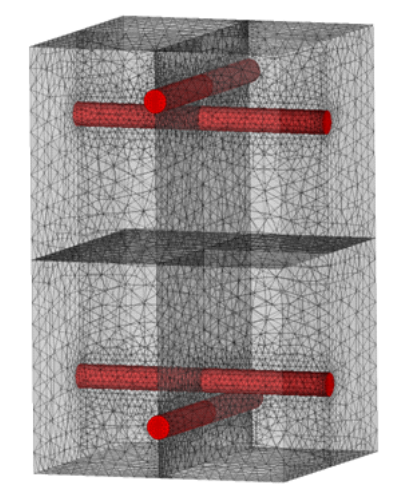
Figure 4 1. Example of a unit RVE mesh for parameters identification (red: steel rebar, grey: concrete) .
An automated*python*™ process automatically generates the RVE mesh from the following eleven geometrical parameters:
Plate thickness |
\(H\) |
|
|
Steel rebar spacing along \({x}_{1}\) and \({x}_{2}\) |
|
|
Diameters of the Four Steel Rebar |
|
|
|
This three-dimensional mesh includes the splitting of nodes located on steel-concrete interfaces (surfaces \({\Gamma }_{b}^{\zeta }\)), the assignment of the different mesh zones to the sub-domains \({\Omega }_{i}^{1}\), \({\Omega }_{i}^{2}\), and periodicity of node locations for the external boundaries (normal unit vectors along \({x}_{1}\) and \({x}_{2}\)). Microscopic material properties and boundary conditions prescribing, including periodicity in the RVE outer surfaces (upper and lower surfaces remaining free) and bond slip basis function are set.
Concerning the ten needed material parameters, the following table gathers the expected values:
2 elastic coefficients for steel |
Young’s modulus, Poisson’s ratio |
\({E}_{s}\), \({\nu }_{s}\) |
2 elastic coefficients for concrete |
Young’s modulus, Poisson’s ratio |
\({E}_{c}\), \({\nu }_{c}\) |
Usual engineering parameters for concrete |
Tensile and compressive strengths, maximum compressive strain, first compressive damage limit |
\({f}_{t}\), \({f}_{c}\),, \({\epsilon }_{\mathrm{cm}}\), \({f}_{\mathrm{dc}}\) |
Steel-concrete sliding experimental pull-out threshold parameter |
\({\tau }_{\mathrm{crit}}\) |
|
Post-peak tensile path parameter of local concrete constitutive relationship |
\({\gamma }_{\text{+}}\) |
They are required in order to perform the \(342\) FEM elastic calculations on the RVE, see the table reported in the Appendix, at section 7.1, and DHRC threshold parameters determination.
The results of the numerical finite element simulations are used to identify the \(335\) DHRC macroscopic parameters with the help of a standard least square algorithm.
Note 20:
In practice, if the obtained values of macroscopic coefficients of \({A}^{\mathrm{mf}}(D)\) , , \(C(D)\) matrices are very small, and making otherwise impossible the parameter identification, we decide to take the corresponding \(\alpha\) , \({\gamma }^{A}\) , ,, , \({\gamma }^{C}\) parameters equal to, * parameters equal to, * parameters equal to \(1\) and \({\gamma }^{B}\) parameters equal to \(0\) .
4.6. Analytical trivial example#
To illustrate the implementation of the previous approach, we take the following representative analytical trivial example.
The first step consists in verifying that the automatic procedure recovers the usual isotropic linear elastic plate stiffness tensor if we take, in the whole RVE, the same uniform sound elastic characteristics (\(E\), \(\nu\)). Indeed, in that case, the RVE \(\Omega\) is reduced to the simple segment \(\text{]}–H/\mathrm{2,}H/2\text{[}\) along the axis \((O{e}_{({x}_{3})})\)), and all the auxiliary fields \({\chi }^{\mathrm{\alpha \beta }}\) in membrane and \({\xi }^{\mathrm{\alpha \beta }}\) in bending depend only on \({x}_{3}\). Solving in such situation the auxiliary problems (3—4), using first trial \(v({x}_{3})\) functions functions \(({v}_{\mathrm{1,}}{v}_{\mathrm{2,}}0)\) then \((\mathrm{0,}\mathrm{0,}{v}_{3})\), we easily obtain:
: label: eq-4
{chi} ^ {mathrm {alphaalpha}} =-frac {nu} {1-nu} (mathrm {0,0}, {x} _ {3})
Hence the macroscopic homogenised elastic plate tensor \(A\) are:
: label: eq-4
{A} _ {mathrm {alphaalphaalphaalpha}}} ^ {mathrm {mm}} =mathrm {EH}/(1- {nu}alphaalphaalphaalphaalphaalphaalpha}}} ^ {2})
4.7. Comparison of parameters with other constitutive models#
In order to give the user comparative information about DHRC parameters, with respect to other constitutive models, like GLRC_DM [R7.01.32], we propose the following evaluation in mono-axial loading cases, first in membrane, then in bending. The information is calculated by the DHRC constitutive model automated identification procedure. So it is more easy to observe the influence of RVE material data on the DHRC parameters, before to perform the structural analysis itself..
4.7.1. Elastic coefficients#
We refer to the GLRC_DMmodel [R7.01.32], § 3.1, to express the RC equivalent elastic moduli in membrane (\({E}_{\mathrm{eq}}^{m}\)) and in bending (\({E}_{\mathrm{eq}}^{f}\)), from material data (concrete \({E}_{b}\), \({\nu }_{b}\) and steel \({E}_{a}\) moduli) and geometrical data (steel section \({S}_{a}\), thickness \(h\), relative position of steel rebar in the thickness \({\chi }_{a}\in \left]\mathrm{0,}1\right[\)):
: label: eq-4
{E} _ {mathrm {eq}}} ^ {m} = {E} _ {a}frac {{S} _ {a}} {h} {h} + {E} _ {b}cdotfrac {{E}} _ {E} _ {e} _ {e}} {b} h+ {E} _ {e} _ {a} {S} _ {a} (1- {nu} _ {b} ^ {2})}
Therefore, the equivalent elastic RC plate coefficients in uniaxial membrane and in uniaxial bending can be deduced by:
: label: eq-4
{A} _ {{mathrm {eq}}} _ {mathrm {GLRC}}}} ^ {0mathrm {mm}} = {E} _ {mathrm {eq}}} ^ {m} h
According to the DHRC formulation in elastic domain, in particular tensor \({A}^{0}\), we can express the membrane stress resulting in uniaxial loading case in terms of membrane uniaxial strain, in both \(x\) and \(y\) steel grids directions, and in the same way for the uniaxial bending case; we get then:
: label: eq-4
left (begin {array} {c} {}}} _ {mathit {xx}} _ {mathit {yy}}\ {}} _ {mathit {xy}}}\ {kappa}}\ {kappa}} _ {mathit {xx}} _ {mathit {xx}}}\ {kappa}}\ {kappa}}\ {kappa}} _ {kappa} _ {mathit {xx}} _ {mathit {xx}} _ {mathit {xx}}}\ {kappa} _ {mathit {xx}} _ {mathit {xx}}}\ {kappa}} _ {mathit {xx}} _ {mathit {xy}}end {array}right) = {left ({mathrm {A}}} ^ {0}right)} ^ {text {-1}}cdotleft (begin {array} {c} {c} {c} {n}} _ {mathit {N}} _ {mathit {x}} _ {mathit {xx}}}\ 0\ 0\ 0\ 0\ 0\ 0\ 0\ 0end {array} {c} {c} {N}} _ {mathit {xx}} _ {mathit {xx}}\ 0\ 0\ 0\ 0\ 0end {array} {left} {c} {c} {
After elimination of all generalised strain variables except respectively \({\epsilon }_{\mathrm{xx}}\) or \({\kappa }_{\mathrm{xx}}\), we easily derive the expressions of the equivalent elastic RC plate coefficients in uniaxial membrane and in uniaxial bending for the DHRC constitutive model, in the \(x\) steel grid direction, in the steel grid direction, to be compared with the closed form GLRC_DM model ones:
: label: eq-4
{A} _ {{mathit {eq}}} _ {mathit {DHRC}}}}} ^ {0mathit {mm}} = {left ({mathrm {A}}} ^ {0}right)} ^ {0}right)}} _ {{mathrm {}}}} _ {{mathrm {}}}} ^ {mathrm {0}right)} _ {{mathrm {0}right)} _ {{mathrm {}}} _ {mathit {xx}}}} ^ {text {-1}}} ^ {-1}}} ^ {0}right)} ^ {0}right)}} ^ {0}right)} ^ {text {-1}}
To be more precise, the same calculations are also performed with the only mixture law contributions to tensor \({A}^{0}\), see section 3.2: this allows to observe the influence of auxiliary fields on final results.
We carry out the same calculations for the \(y\) steel grid direction.
4.7.2. Post-elastic coefficients#
In order to check the post-elastic response of the DHRC constitutive model, we calculable at the state \(D=0\) and \(\dot{D}>0\) the rate of stress resultants in radial monoaxial loading paths in respect of the rate of generalized strain variables, provided we have distinguished compressive then tensile cases for membrane loading. According to relationships (3.2-11) and (3.2.12):
: label: eq-4
(begin {array} {}dot {N}}\ dot {N}\ dot {M}\ dot {M}end {array}) =left [begin {array} {cc} {A} ^ {0mathrm {mm}}} & {A}}\dot {M}}\ dot {M}}\ end {array}}) =left [begin {array} {cc} {A} {A} ^ {0mathrm {mm}}} & {A} ^ {0mathrm {mm}}} & {A} ^ {0mathrm {mm}}} & {A} ^ {0mathrm {mm}}} & {A} ^ {0mathrm {mm}}} & {A} ff}}end {array}right]: (begin {array} {}dot {E}\ dot {K}end {array}) +dot {D}right]: (begin {array}): (begin {array}right]: (begin {array} {}): (begin {array}}: (begin {array}): (begin {array}): (begin { left [begin {array} {cc} {A} _ {, D} _ {, D} _ {, D} _ {, D} ^ {mathrm {mf}} (0)\ {A} _ {, D} _ {, D} ^ {mathrm {fm}}} (0) & {A} _ {, D}} ^ {mathrm {fm}} (0) & {A} _ {, D}} ^ {mathrm {fm}}} (0) & {A} _ {, D}} ^ {mathrm {fm}}} (0)} (0)end {array}right]: (begin {array} {} E\ Kend {array})
According to (4.4-2), we recall that derivatives \({A}_{,D}(0)\) are directly dependent on tensor \({A}^{0}\) and \({\alpha }^{A}\) and \({\gamma }^{A}\) parameters, respectively in a tensile, compressive membrane, or positive or negative bending state. Moreover, the consistency conditions \({\dot{f}}_{({d}^{\rho })}=0\) give:
: label: eq-4
dot {D} =frac {-2 (begin {array} {} {} E\ Kend {array}):left [begin {array} {cc} {A} _ {, D} ^ {mathrm {mm}} ^ {mathrm {mm}}} ^ {mathrm {mm}} ^ {mathrm {mm}}} ^ {mathrm {mm}}} ^ {mathrm {mm}}} (0) {mathrm {mm}}} ^ {mathrm {mm}}} (0) {mathrm {mm}}} ^ {mathrm {mm}}} (0) {mathrm {mm}}} (0) {mathrm {mm}}} ^ {{mathrm {fm}} (0) & {A} _ {, D} _ {, D} ^ {mathrm {ff}} (0)end {array} {}dot {E}dot {E}\ dot {E}\ dot {E}\ dot {E}\ dot {E}\ dot {E}\ dot {E}\ dot {E}\ dot {E}\ dot {E}\ dot {E}\dot {E}\ dot {E}\ dot {E}\ dot {E}\ dot {E}\ dot {E}\ dot {E}\ dot {E}\ dot {E}\ dot {E}\ dot {E}\ dot {E}\ {array} {cc} {A} _ {,mathrm {DD}}} ^ {mathrm {mm}} (0) & {A} _ {,mathrm {DD}}} ^ {mathrm {mf}}} (0) (0)\ mathrm {fm}}} ^ {mathrm {fm}}} ^ {mathrm {fm}}} ^ {mathrm {fm}}} ^ {mathrm {fm}}} ^ {mathrm {fm}}} ^ {mathrm {fm}}} ^ {mathrm {fm}}} (0) & {A} _ {,mathrm {DD}}} ^ {mathrm {ff}} (0)end {array}right]: (begin {array} {}} E\ Kend {ff}}}
As we consider radial loading paths controlled by a regular \(h(t)\) function, we can write:
: label: eq-4
(begin {array} {}dot {E}\ dot {E}\ dot {E}\ dot {K}end {array}) =dot {h} (t)mathrm {.} (begin {array} {} {E} _ {1}\ {K} _ {1}end {array})
So we can write the rate equations in a concise manner:
: label: eq-4
(begin {array} {}dot {N}}\ dot {N}\ dot {M}\ dot {M}end {array}) =left [begin {array} {cc} {A} ^ {Tmathrm {mm}}} & {A}} {A} ^ {A} ^ {A} ^ {A} ^ {Tmathrm {fm}}} ^ {A} ^ {Tmathrm {fm}}} & {A} ^ {A} ^ {Tmathrm {fm}}} & {A} ^ {Tmathrm {mm}}} & {A} ^ {Tmathrm {mm}}} & {A} ^ {Tmathrm {mm}}} & {A} ^ {A}} {ff}}end {array}right]: (begin {array} {}dot {E}\ dot {K}end {array}end {array})
Where tensor \({A}^{T}\) results from contribution of \({A}^{0}\) and their derivatives at \(D=0\), see equations (4.7-5) and (4.7-6) applied for the directions \(({E}_{1},{K}_{1})\). And we apply to tensor \({A}^{T}\) the same procedure than done for tensor \({A}^{0}\) at section 4.7.1 to calculate the equivalent post-elastic RC plate rate coefficients in uniaxial membrane (compressive then tensile cases) and in uniaxial bending for the DHRC constitutive model, in the constitutive model, in the \(x\) steel grid direction, then in \(y\) steel grid direction.
We refer to the GLRC_DM model [R7.01.32], § 3.2.2.1 and § 3.2.2.3, to express the RC equivalent post-elastic rate coefficients in membrane and in bending, I order to make comparison with DHRC constitutive model. We can also prefer to make this comparison with asymptotic slopes of membrane and bending responses of GLRC_DM model, see [R7.01.32], § 3.2.3.1 and § 3.2.3.3. Nevertheless, we can adopt the simplified expressions given in [R7.01.32], § 3.2.4.1 and § 3.2.4.3, involving \({\gamma }_{\mathrm{mt}}\), \({\gamma }_{\mathrm{mc}}\), \({\gamma }_{f}\) GLRC_DMparameters, acting as proportional reduction factors on elastic coefficients.
4.8. Internal Variables of the DHRC Model#
The internal variables output of*Code_Aster* are the following: the six fist are true thermodynamic internal variables, the five last ones are produced for easier post-treatment.
variables |
name |
contents |
\(\mathrm{V1}\) |
“ENDOSUP” |
\({D}_{1}\) Damage in the upper half of RVE |
\(\mathrm{V2}\) |
“ENDOINF” |
\({D}_{2}\) Damage in the lower half of RVE |
\(\mathrm{V3}\) |
“GLISXSUP” |
\({E}_{x}^{\eta 1}\) bond sliding of \(x\) rebar in the upper half of RVE |
\(\mathrm{V4}\) |
“GLISYSUP” |
\({E}_{y}^{\eta 1}\) bond sliding of \(y\) rebar in the upper half of RVE |
\(\mathrm{V5}\) |
“GLISXINF” |
\({E}_{x}^{\eta 2}\) bond sliding of \(x\) rebar in the lower half of RVE |
\(\mathrm{V6}\) |
“GLISYINF” |
\({E}_{y}^{\eta 2}\) bond sliding of \(y\) rebar in the lower half of RVE |
\(\mathrm{V7}\) |
“DISSENDO” |
Dissipated energy by damage: \({D}_{\mathrm{diss}}^{\mathrm{endo}}(t)={G}_{1}^{\mathrm{crit}}{D}_{1}(t)+{G}_{2}^{\mathrm{crit}}{D}_{2}(t)\) |
\(\mathrm{V8}\) |
“DISSGLIS” |
Dissipated energy by bond sliding: \(\begin{array}{}{D}_{\mathrm{diss}}^{\mathrm{bond}-\mathrm{slide}}(t)=\text{}\\ {\Sigma }_{x}^{\mathrm{crit}1}{\int }_{0}^{t}{\dot{E}}_{x}^{\eta 1}\mathrm{dt}+{\Sigma }_{y}^{\mathrm{crit}1}{\int }_{0}^{t}{\dot{E}}_{y}^{\eta 1}\mathrm{dt}+{\Sigma }_{x}^{\mathrm{crit}2}{\int }_{0}^{t}{\dot{E}}_{x}^{\eta 2}\mathrm{dt}+{\Sigma }_{y}^{\mathrm{crit}2}{\int }_{0}^{t}{\dot{E}}_{y}^{\eta 2}\mathrm{dt}\end{array}\) |
\(\mathrm{V9}\) |
“DISSIP” |
Sum of both energy dissipations |
\(\mathrm{V10}\) |
“ADOUMEMB” |
Mean relative weakening of membrane stiffness of reinforced concrete slab |
\(\mathrm{V11}\) |
“ADOUFLEX” |
Mean relative weakening of bending stiffness of reinforced concrete slab |
Distinction between upper and lower faces is made from the orientation of the local reference frame at each Gauss” Point. So, the lower face is damaged \(\dot{{D}_{2}}>0\) for positive plate increasing curvatures, whereas the upper one is damaged \(\dot{{D}_{1}}>0\) for negative curvatures.
The \(\mathrm{V10}\) and \(\mathrm{V11}\) values are comparable to the equivalent scalar variables being produced by the GLRC_DM model, see [R7.01.32], to roughly describe the stiffness degradation of the RC plate. The respective calculated expressions are at each time-step:
: label: eq-4
mathrm {V10} =1-sqrt [3] {{A}} _ {mathrm {xxxx}} ^ {mathrm {mm}} (D) {A} _ {mathrm {yyyy}}}} ^ {mathrm {yyyy}}} ^ {mathrm {yyyy}}} ^ {mathrm {yyyy}}} ^ {mathrm {yyyy}}} ^ {mathrm {yyyy}}} ^ {mathrm {yyyy}}} ^ {mathrm {yyyy}}} ^ {mathrm {yyyy}}} ^ {mathrm {yyyy}}} ^ {mathrm {yyyy}}} ^ {mathrm {yyyy} (D)}/sqrt [3] {{A} _ {mathrm {xxxx}}} ^ {mathrm {0mm}} {A} _ {mathrm {yyyy}}} ^ {mathrm {yyyy}}} ^ {mathrm {yyyy}}} ^ {mathrm {yyyy}}} ^ {mathrm {yyyy}}} ^ {mathrm {yyyy}}} ^ {mathrm {yyyy}}} ^ {mathrm {yyyy}}} ^ {mathrm {yyyy}}} ^ {mathrm {yyyy}}} ^ {mathrm {yyyy}}} ^ {mathr mathrm {V11} =1-sqrt [3] {{A}} _ {mathrm {xxxx}} ^ {mathrm {ff}} (D) {A} _ {mathrm {yyyy}}} {mathrm {yyyy}}} ^ {mathrm {yyyy}}} ^ {mathrm {yyyy}}} ^ {mathrm {yyyy}}} ^ {mathrm {yyyy}}} ^ {mathrm {yyyy}}} ^ {mathrm {yyyy}}} ^ {mathrm {yyyy}}} ^ {mathrm {yyyy}}} ^ {mathrm {yyyy}}} ^ {mathrm {yyyy}}} (D)}/sqrt [3] {{A} _ {mathrm {xxxx}}} ^ {mathrm {0ff}} {A} _ {mathrm {yyyy}}}} ^ {mathrm {yyyy}}} ^ {mathrm {yyyy}}} ^ {mathrm {yyyy}}} ^ {mathrm {yyyy}}} ^ {mathrm {yyyy}}} ^ {mathrm {yyyy}}} ^ {mathrm {yyyy}}} ^ {mathrm {yyyy}}} ^ {mathrm {yyyy}}} ^ {mathrm {yyyy}}}} ^ {
They are being zero in absence of damage. These two variables neglect membrane-bending coupling.