2. The MAZARS models#
2.1. Original Mazars Model#
The MAZARS model was developed as part of damage mechanics. This model is detailed in the thesis of MAZARS]
The constraint is given by the following relationship:
: label: EQ-None
sigma = (1-D)text {E} {epsilon} ^ {mathrm {e}}
with:
\(E\) the Hooke matrix,
\(D\) the damage variable
\({\varepsilon }^{e}\) elastic deformation \({\varepsilon }^{e}=\varepsilon -{\varepsilon }^{\text{th}}-{\varepsilon }^{\text{rd}}-{\varepsilon }^{\text{re}}\)
• \({\varepsilon }^{\text{th}}=\alpha (T-{T}_{\text{ref}}){I}_{d}\) thermal expansion
• \({\varepsilon }^{\text{re}}\mathrm{=}\mathrm{-}\beta \xi {\mathrm{I}}_{\mathrm{d}}\) endogenous withdrawal (linked to hydration)
• \({\varepsilon }_{\text{rd}}=-\kappa ({C}_{\text{ref}}-C){I}_{d}\) desiccation shrinkage (related to drying)
\(D\) is the damage variable. It is between \(0\), healthy material, and \(1\), broken material. The damage is driven by equivalent deformation \({\epsilon }_{\text{eq}}\), which makes it possible to translate a triaxial state into an equivalence to a uniaxial state. As extensions are essential in the phenomenon of concrete cracking, the equivalent deformation introduced is defined on the basis of the positive eigenvalues of the deformation tensor, i.e.:
\({\epsilon }_{\text{eq}}=\sqrt{{\langle \epsilon \rangle }_{+}\mathrm{:}{\langle \epsilon \rangle }_{+}}\) where in the main coordinate system of the deformation tensor: \({\varepsilon }_{\text{eq}}=\sqrt{{\langle {\varepsilon }_{1}\rangle }_{+}^{2}+{\langle {\varepsilon }_{2}\rangle }_{+}^{2}+{\langle {\varepsilon }_{3}\rangle }_{+}^{2}}\) |
(eq 2.1-2 ) |
knowing that the positive part \({\mathrm{\langle }\mathrm{\rangle }}_{+}\) is defined so that if \({\varepsilon }_{i}\) is the main deformation in the direction \(i\):
: label: EQ-None
{begin {array} {c} {langle {epsilon} _ {i}epsilon} _ {+} = {epsilon} _ {i}text {epsilon} _ {epsilon} _ {i}epsilon} _ {i}epsilon} _ {epsilon} _ {+} =0text {epsilon} _ {epsilon} _ {+} =0text {epsilon} _ {epsilon} _ {+} =0text {epsilon} _ {epsilon} _ {+} =0text {epsilon} _ {epsilon} _ {+} =0text {epsilon} _ {epsilon} _ {silon} _ {i} <0end {array}
Note:
In the case of thermo-mechanical loading, only elastic deformation \({\varepsilon }^{e}\mathrm{=}\varepsilon \mathrm{-}{\varepsilon }^{\text{th}}\) contributes to the evolution of the damage, whence: \({\varepsilon }_{\text{eq}}\mathrm{=}\sqrt{{\mathrm{\langle }{\varepsilon }^{e}\mathrm{\rangle }}_{+}\mathrm{:}{\mathrm{\langle }{\varepsilon }^{e}\mathrm{\rangle }}_{+}}\) .
\({\epsilon }_{\text{eq}}\) is an indicator of the state of tension in the material that is causing the damage. This quantity defines the load area \(f\) as:
: label: EQ-None
fmathrm {=} {varepsilon} _ {text {eq}}mathrm {-} K (D)mathrm {=} 0
(4)
with \(K(D)={\epsilon }_{\text{d0}}\) if \(D=0\). \({\epsilon }_{\text{d0}}\) the deformation damage threshold.
When the equivalent deformation reaches this value, the damage is activated. \(D\) is defined as a combination of two damage modes defined by \({D}_{\text{t}}\) and \({D}_{\text{c}}\), varying between 0 and 1 depending on the associated damage state, and corresponding to tensile and compressive damage respectively. The relationship between these variables is as follows:
: label: EQ-None
Dmathrm {=} {alpha} _ {t} _ {t} ^ {beta} {D} _ {t} + {alpha} _ {c} ^ {beta} {beta} {D} {D} _ {c}
(5)
\(\beta\) is a coefficient that was introduced later to improve shear behavior. Usually its value is fixed at 1.06. The coefficients \({\alpha }_{\text{t}}\) and \({\alpha }_{\text{c}}\) establish a link between the damage and the state of tension or compression. When traction is activated \({\alpha }_{\text{t}}=1\) while \({\alpha }_{\text{t}}=0\) and vice versa in compression.
A particularity of this model is its explicit writing, which implies that all the quantities are calculated directly without using a linearization algorithm such as that of Newton-Raphson. Thus, the laws of evolution of damages \({D}_{\text{t}}\) and \({D}_{\text{c}}\) are expressed only on the basis of the equivalent deformation \({\epsilon }_{\text{eq}}\)
: label: EQ-None
{D} _ {t}mathrm {=}} 1mathrm {-}frac {(1mathrm {-} {A} _ {t}) {varepsilon} _ {mathit {d0}}} {mathit {d0}}} {mathit {d0}}}} {mathit {d0}}}} {mathit {d0}}}} {mathit {d0}}}} {mathit {d0}}}} {mathit {d0}}}} {mathit {d0}}}} {mathit {d0}}}} {mathit {d0}}}} {mathit {d0}}}} {mathit {d0}text {exp} (mathrm {-} {B}} _ {B} _ {t} ({varepsilon} _ {text {eq}}mathrm {-} {varepsilon} {varepsilon}} _ {varepsilon} _ {mathit {d0}}})
: label: EQ-None
{D} _ {c}mathrm {=}} 1mathrm {-}frac {(1mathrm {-} {A} _ {c}) {varepsilon} _ {mathit {d0}}} {mathit {d0}}}} {mathit {d0}}}} {mathit {d0}}}} {mathit {d0}}}} {mathit {d0}}}} {mathit {d0}}}} {mathit {d0}}}} {mathit {d0}}}} {mathit {d0}}}} {mathit {d0}}}} {mathit {d0}}}} {mathit {d0text {exp} (mathrm {-} {B}} _ {B} _ {c} ({varepsilon} _ {text {eq}}mathrm {-} {varepsilon} {varepsilon}} _ {varepsilon} _ {mathit {d0}}})
with \({A}_{t}\), \({A}_{c}\), \({B}_{t}\), and \({B}_{c}\), material parameters to be identified. These parameters make it possible to modulate the shape of the post-peak curve. They are obtained using tensile tests and a compression test.
2.2. Mazars Revisited Model#
Although commonly used, the Mazars Origin model has shortcomings in modeling the behavior of concrete during shear and bi-compression loading. A comparison between the load surfaces of the two models is given in.
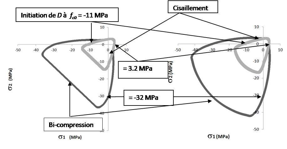
a) Original Mazars Model b) Revisited Mazars Model
Figure 2.2-1: Comparison of damage initiation and failure surfaces of Mazars models in plane \({\sigma }_{3}=0\) and C30 concrete
Thus, a new formulation is proposed through 2 major modifications:
improvement of bi-compression behavior,
simplification and improvement of shear behavior.
The original Mazars model [from the 1980s] greatly underestimates the strength of concrete under bi-compression. The first modification made by the Revisited model therefore improves the bi-compression behavior. This goal is achieved by correcting the equivalent deformation when at least one main stress is negative, using a variable \(\gamma\):
: label: EQ-None
{epsilon} _ {mathit {eq}}} ^ {mathit {corrected}} =gamma {epsilon} _ {text {eq}} =gammasqrt {{langleepsilonrangle}} ^ {langleepsilonrangle}} ^ {langleepsilonrangle}}} ^ {langleepsilonrangle}} ^ {langleepsilonrangle}} ^ {langleepsilonrangle}} ^ {langleepsilonrangle}} ^ {langleepsilonrangle}} ^ {mathit {eq}} ^ {mathit {eq}}
with:
: label: EQ-None
{begin {array} {c}gamma =-frac {sqrt {sqrt {sqrt {sum _ {i} {sigma}}} _ {i}rangle} _ {-}rangle} _ {-}} _ {-} ^ {2}}} {-} ^ {2}}}}} {sum _ {2}}}} {sum _ {i} {2}}}} {sum _ {i} {2}}}} {sum _ {i} {2}}}} {sum _ {i} {i} {2}}}} {sum _ {i} {2}}}} {sum _ {i} {i} {2}}}} {sum _ {i} {2}}}} _ {-}}text {if at least one effective constraint is negative}\gamma =1text {otherwise}end {array}
The effective stress in the sense of the mechanics of damage is defined by:
: label: EQ-None
underline {underline {tilde {sigma}}}}mathrm {=}frac {underline {underline {sigma}}} {1mathrm {sigma}}} {1mathrm {-} D}
The definition of < > - is similar to:
: label: EQ-None
{begin {array} {c} {langle {stackrel {stackrel {}} {sigma}} _ {i}rangle} _ {-} = {stackrel {} {sigma}}} _ {sigma}} _ {sigma}} = {i}le 0\ {sigma}} _ {langle {stackrel}} _ {langle {stackrel {}}} {sigma}} _ {i}rangle}} _ {-} = 0text {sigma} {sigma}} _ {i} >0end {array} >0end {array}
where \({\tilde{\sigma }}_{i}\) is a primary effective constraint.
The improvement of shear behavior is achieved by the introduction of a new internal variable: \(Y\). It corresponds to the maximum reached during the loading of the equivalent deformation. Its initial value \({Y}_{0}\) is \({\epsilon }_{\mathit{d0}}\). \(Y\) is defined by the following equation:
: label: EQ-None
Y=text {max}left ({epsilon}} _ {mathit {d0}}}text {, max}left ({epsilon} _ {mathit {eq}}}} ^ {mathit {eq}}} ^ {mathit {eq}}} ^ {mathit {eq}}} ^ {mathit {eq}}} ^ {mathit {corrected}}right)right)
The charging function is:
: label: EQ-None
f= {epsilon} _ {mathit {eq}}} ^ {mathit {corrected}} -Y
The evolution of the damage is given by:
: label: EQ-None
Dmathrm {=} 1mathrm {-}frac {(1mathrm {-} A) {Y} _ {0}} {Y}mathrm {-} Atext {exp} (text {exp}} (mathrm {-}})
In this expression, it is the variables \(A\) and \(B\) that make it possible to reproduce the almost fragile behavior of concrete under tension and the work-hardened behavior under compression. To best represent the experimental results, the following laws of evolution were chosen for \(A\) and \(B\):
: label: EQ-None
Amathrm {=} {A} _ {t} ({mathrm {2r}}} ^ {2} (1mathrm {-}mathrm {2k})mathrm {-} r (1mathrm {-} r (1mathrm {-}mathrm {-}}mathrm {2r}} r (1mathrm {-} r (1mathrm {-} r (1mathrm {-}} r (1mathrm {-} r (1mathrm {-}) r (1mathrm {-} r (1mathrm {-} r (1mathrm {-} r (1mathrm {-} r (1mathrm}mathrm {-}mathrm {3r} +1)
and
: label: EQ-None
Bmathrm {=} {r} ^ {2} {2} {B} {B} _ {t} + (1mathrm {-} {r} ^ {2}) {B} _ {2}) {B} _ {c}
where the expression for \(r\) is:
: label: EQ-None
r=frac {sum _ {i} {langle {stackrel {stackrel {}} {sigma}} _ {i}rangle} _ {+}} {sum _ {i}mid}mid}mid}mid}mid}mid}mid}
In these equations, a new variable \(r\) appears, which tells us about the stress state. When \(r\) is equal to 1 (corresponding to the traction sector), the variables \(A\) and \(B\) are equivalent to the parameters \({A}_{t}\) and \({B}_{t}\). So is the same as. Conversely, if \(r\) is zero (corresponding to the compression sector), then \(A={A}_{c}\), \(B\mathrm{=}{B}_{c}\) and is the same as.
In plan \({\sigma }_{3}=0\), the evolution according to the sign of the main constraints of the variables \(A\), \(B\), \(r\) and \(\gamma\) depends on the sign of the main constraints.
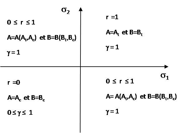
Figure 2.2-2: Evolution of the variables \(A\), \(B\),, \(r\) and \(\gamma\) in the \({\sigma }_{3}\mathrm{=}0\) plane
In the equation a new parameter appears: \(k\). It introduces an asymptote to curve \(\sigma -\epsilon\) in shear and is defined by:
: label: EQ-None
kmathrm {=}frac {{A} _ {text {shear}}} {{A} _ {t}}
where \({A}_{\text{cisaillement}}\) defines residual stress in pure shear. It is similar to \({A}_{t}\) for this load case. The recommended value for \(k\) is \(0.7\). The value of \(k\) less than 1 is very useful in modeling the effects of friction between concrete and reinforcements in reinforced concrete structures because it induces residual shear stress. For the value \(k=1\) we find the behavior of the Original model ().
Asymptote induced by k 1
Figure 2.2-3: Stress-strain curve during a pure shear test on a Gauss point
The Origin model underestimates the strength of concrete under pure shear. This new formulation makes it possible to increase this pure shear strength from \(2.5\mathit{MPa}\) to \(3.5\mathit{Mpa}\) for C30 concrete. This value depends on those of the material parameters entered (\({A}_{t}\), \({A}_{c}\), \({B}_{t}\), and \({B}_{c}\)).
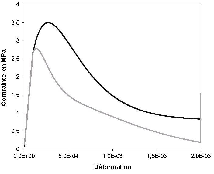
The local response of the Mazars Revisited model under successive tensile and compression loading is given by the.
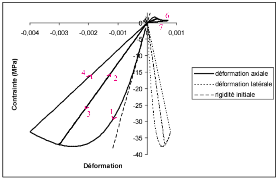
Figure 2.2-4: Stress-strain response of the Mazars model for 1D stress.
It allows you to visualize a certain number of characteristics of the Mazars model, namely:
the damage affects the stiffness of the concrete,
there are no irreversible deformations,
the tensile and compression responses are well asymmetric,
Note: The Mazars Original and Revisited models do not take into account the unilateral nature of concrete, namely the closure of cracks during the transition from a state of tension to a state of compression.