3. Identification#
In addition to thermo-elastic parameters \(E,\nu ,\alpha\), the MAZARS Revisited model involves 6 material parameters: \({A}_{c},{B}_{c},{A}_{t},{B}_{t},{\varepsilon }_{\mathit{d0}},k\).
\({\varepsilon }_{\mathrm{d0}}\) is the damage threshold. It obviously acts on the peak stress but also on the shape of the post-peak curve. In fact, the drop in stress is all the less sudden the smaller \({\varepsilon }_{\mathrm{d0}}\) is. In general \({\varepsilon }_{\mathrm{d0}}\) is included in \(0.5\) and \(1.5{10}^{\mathrm{-}4}\).
The coefficients \(A\) and \(B\) make it possible to modulate the shape of the post-peak curve. They are defined by the equations and depend on the parameters of the Mazars Origin Model (\({A}_{t}\), \({B}_{t}\), \({A}_{c}\) and \({B}_{c}\)) and on \(r\):
\(A\) introduces a horizontal asymptote which is the \(\varepsilon\) axis for \(A\mathrm{=}1\) and the horizontal passing through the peak for \(A\mathrm{=}0\) (cf. []). In the field of traction, \(A\) is equivalent to \({A}_{t}\) (and vice versa in the field of compressions \(A={A}_{c}\)). In general, \({A}_{c}\) is between 1 and 2. and \({A}_{t}\) between 0.7 and 1.
\(B\) depending on its value can correspond to a sudden drop in stress (\(B>10000\)) or a preliminary phase of stress increase followed, after passing through a maximum, by a more or less rapid decrease as can be seen on the []. In the field of traction, \(B\) is equivalent to \({B}_{t}\) (and vice versa in the field of compressions \(B={B}_{c}\)). In general \({B}_{c}\) is between \(1000\) and \(2000\) and \({B}_{t}\) between \(9000\) and \(21000\).
\(k\) introduces a horizontal asymptote in pure shear on the stress-strain curve if its value is different from 1 for \({A}_{t}=1\),. The recommended value is \(0.7\).
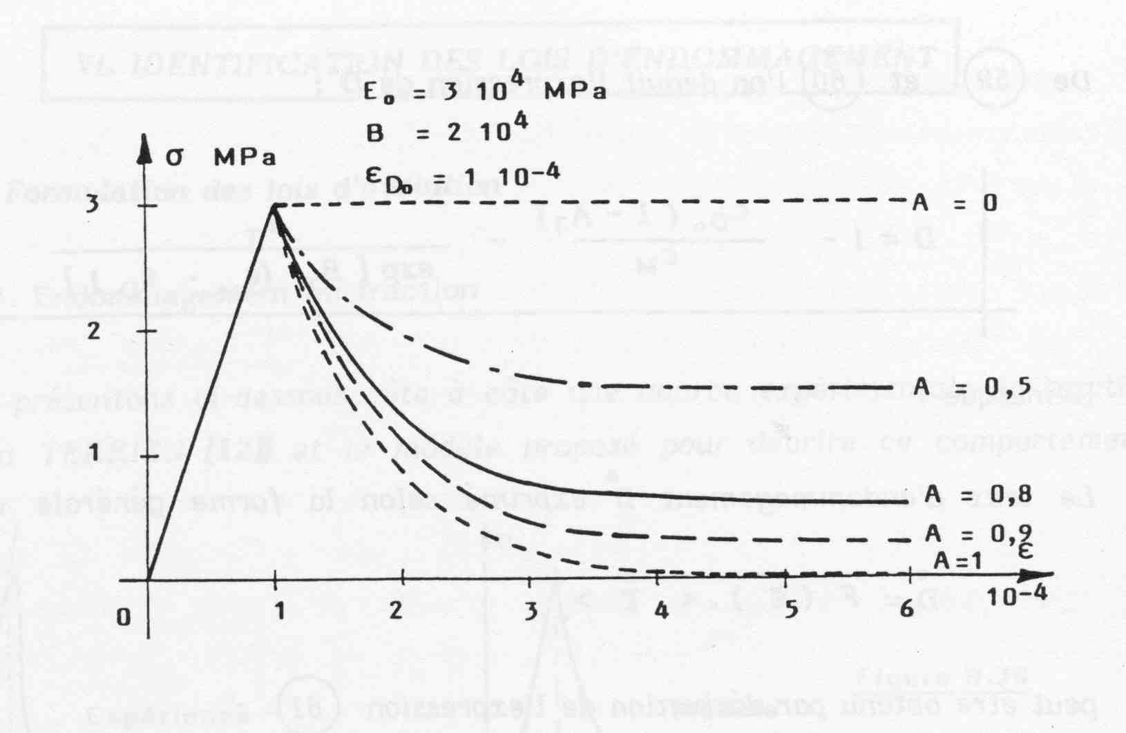
Fig figure 3-1: Influence of the parameter \({A}_{t}\)
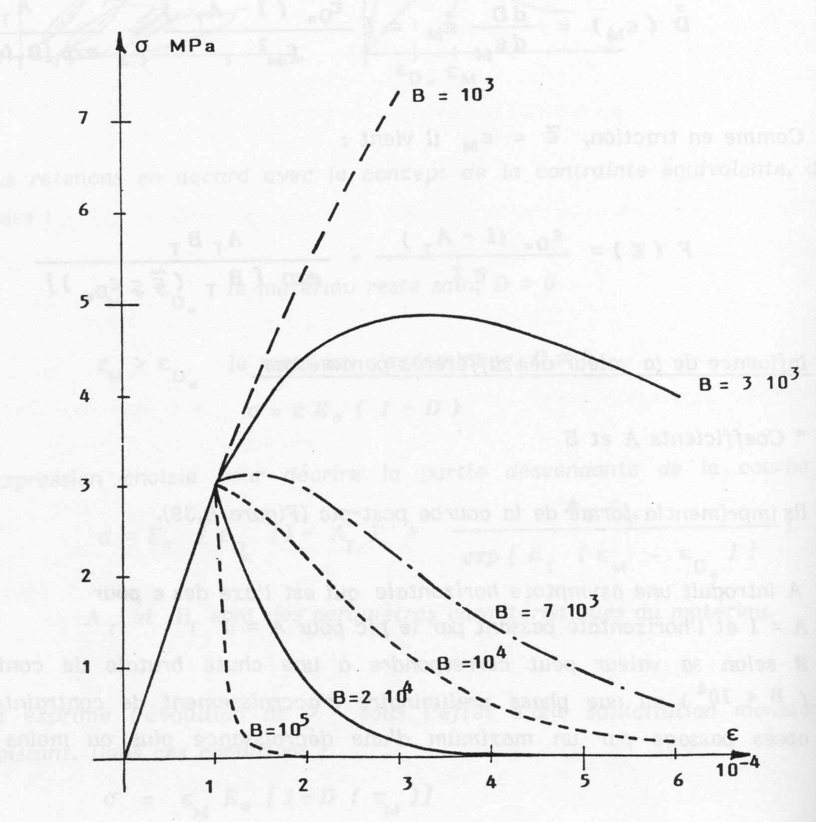
Fig ure 3-2: Influence of the parameter \({B}_{t}\)
One way to obtain a set of parameters is to have the results of uniaxial compression and tension tests available (for traction, other types of tests can be used, « Brazilian » splitting tests for example).
If deformation gradient regularization is used (see § 1.2), it is recommended to set the parameters of the law at the same time as the characteristic length \({L}_{c}\). Some authors (confer) also suggest calibrating \({L}_{c}\) by using experimental tests on several sizes of specimens; in fact, the characteristic length is linked to the size of the energy dissipation zone which could be at the origin of structural scale effects.