4. Discretization of the equations constituting the model

4.1. Discretization of the constitutive equations of spherical creep

A first-order linearization of the product of stresses and humidity is carried out:

\(\sigma (t)\cdot h(t)\approx {\sigma }_{n}\cdot {h}_{n}+\frac{t-{t}_{n}}{{\mathrm{\Delta t}}_{n}}({\mathrm{\Delta \sigma }}_{n}\cdot {h}_{n}+{\sigma }_{n}\cdot {\mathrm{\Delta h}}_{n})\) eq 4.1-1

After discretizing the stresses and the relative humidity by affine functions, the spherical natural creep deformation is discretized by the following equation:

\({\text{Δε}}_{n}^{\text{fs}}={a}_{n}^{s}+{b}_{n}^{s}\cdot {\sigma }_{n}^{s}+{c}_{n}^{s}\cdot {\sigma }_{n+1}^{s}\iff \Delta \left(\text{tr}{\underline{\underline{\epsilon }}}^{f}\right)={\mathrm{3a}}_{n}^{s}+{b}_{n}^{s}\cdot \text{tr}{\underline{\underline{\sigma }}}_{n}+{c}_{n}^{s}\cdot \text{tr}{\underline{\underline{\sigma }}}_{n+1}\) eq 4.1-2

where \({\sigma }_{n}^{s}\) and \({\sigma }_{n+1}^{s}\) are the spherical constraints at the start and end of the current time step.

It is necessary to distinguish two scenarios depending on whether the irreversible deformation must be taken into account or not.

1st case: irreversible spherical creep deformation is not taken into account, the equation [éq4.1‑2] can be put in the form (simple Kelvin chain):

\({\eta }_{r}^{s}{\dot{\epsilon }}_{r}^{\text{fs}}(t)+{k}_{r}^{s}{\epsilon }_{r}^{\text{fs}}(t)=h(t){\sigma }_{r}^{s}(t)\) eq 4.1-3

After discretization, the previous equation can be put in the form:

\({\text{Δε}}_{r,n}^{\text{fs}}={a}_{r,n}^{s}+{b}_{r,n}^{s}\cdot {\sigma }_{n}^{s}+{c}_{r,n}^{s}\cdot {\sigma }_{n+1}^{s}\) eq 4.1-4

With:

\(\{\begin{array}{c}{a}_{r,n}^{s}=\left[\text{exp}(-\frac{{\mathrm{\Delta t}}_{n}}{{\tau }_{r}^{s}})-1\right]\cdot {\epsilon }_{r,n}^{\text{fs}}\\ {b}_{r,n}^{s}=\frac{1}{{k}_{r}^{s}}\left\{\left[-(\frac{{\mathrm{2\tau }}_{r}^{s}}{{\mathrm{\Delta t}}_{n}}+1){h}_{n}+\frac{{\tau }_{r}^{s}}{{\mathrm{\Delta t}}_{n}}{h}_{n+1}\right]\text{exp}(-\frac{{\mathrm{\Delta t}}_{n}}{{\tau }_{r}^{s}})+\left[(\frac{{\mathrm{2\tau }}_{r}^{s}}{{\mathrm{\Delta t}}_{n}}-1){h}_{n}-\frac{{\tau }_{r}^{s}-{\mathrm{\Delta t}}_{n}}{{\mathrm{\Delta t}}_{n}}{h}_{n+1}\right]\right\}\\ {c}_{r,n}^{s}=\frac{1}{{k}_{r}^{s}}\left[\frac{{\tau }_{r}^{s}}{{\mathrm{\Delta t}}_{n}}\text{exp}(-\frac{{\mathrm{\Delta t}}_{n}}{{\tau }_{r}^{s}}){h}_{n}-\frac{{\tau }_{r}^{s}-{\mathrm{\Delta t}}_{n}}{{\mathrm{\Delta t}}_{n}}{h}_{n}\right]\end{array}\) eq 4.1-5

As for the irreversible deformation, it does not vary:

\({\text{Δε}}_{i,n}^{\text{fs}}=0\Rightarrow \{\begin{array}{c}{a}_{i,n}^{s}=0\\ {b}_{i,n}^{s}=0\\ {c}_{i,n}^{s}=0\end{array}\) eq 4.1-6

2ndcas: irreversible spherical creep deformation must be taken into account.

Using linearization [éq 4.1-1],], the system of coupled equations is written:

\(\{\begin{array}{c}{\dot{\epsilon }}_{r}^{\text{fs}}(t)+2{\dot{\epsilon }}_{i}^{\text{fs}}(t)=\frac{1}{{\eta }_{r}^{s}}\left[{\sigma }_{n}\cdot {h}_{n}+\frac{t-{t}_{n}}{{\mathrm{\Delta t}}_{n}}({\mathrm{\Delta \sigma }}_{n}\cdot {h}_{n}+{\sigma }_{n}\cdot {\mathrm{\Delta h}}_{n})-{k}_{r}^{s}{\epsilon }_{r}^{\text{fs}}(t)\right]\\ {\dot{\epsilon }}_{i}^{\text{fs}}(t)=-\frac{1}{{\eta }_{i}^{s}}(-{\mathrm{2k}}_{r}^{s}{\epsilon }_{r}^{\text{fs}}(t)+{k}_{i}^{s}{\epsilon }_{i}^{\text{fs}}(t)+{\sigma }_{n}\cdot {h}_{n}+\frac{t-{t}_{n}}{{\mathrm{\Delta t}}_{n}}({\mathrm{\Delta \sigma }}_{n}\cdot {h}_{n}+{\sigma }_{n}\cdot {\mathrm{\Delta h}}_{n}))\end{array}\) eq 4.1-7

This system can take the form of:

\({\underline{\dot{\epsilon }}}^{\text{fs}}(t)=\left[\begin{array}{c}{\dot{\epsilon }}_{r}^{\text{fs}}(t)\\ {\dot{\epsilon }}_{i}^{\text{fs}}(t)\end{array}\right]=\underline{\underline{A}}:{\underline{\epsilon }}_{r}^{\text{fs}}(t)+\underline{b}+(t-{t}_{n})\underline{c}\iff \{\begin{array}{c}{\dot{\epsilon }}_{r}^{\text{fs}}(t)={a}_{\text{rr}}^{s}{\epsilon }_{r}^{\text{fs}}(t)+{a}_{\text{ri}}^{s}{\epsilon }_{i}^{s}(t)+{b}_{r}^{s}+{c}_{r}^{s}(t-{t}_{n})\\ {\dot{\epsilon }}_{i}^{\text{fs}}(t)={a}_{\text{ir}}^{s}{\epsilon }_{r}^{\text{fs}}(t)+{a}_{\text{ii}}^{s}{\epsilon }_{i}^{s}(t)+{b}_{i}^{s}+{c}_{i}^{s}(t-{t}_{n})\end{array}\) eq 4.1-8

\(\underline{\underline{A}}\), \(\underline{b}\), and \(\underline{c}\) are defined as follows:

\(\begin{array}{}\underline{\underline{A}}=\left[\begin{array}{cc}{a}_{\text{rr}}^{s}& {a}_{\text{ri}}^{s}\\ {a}_{\text{ir}}^{s}& {a}_{\text{ii}}^{s}\end{array}\right]=\left[\begin{array}{cc}-\frac{{k}_{r}^{s}}{{\eta }_{r}^{s}}-4\frac{{k}_{r}^{s}}{{\eta }_{i}^{s}}& 2\frac{{k}_{i}^{s}}{{\eta }_{i}^{s}}\\ 2\frac{{k}_{r}^{s}}{{\eta }_{i}^{s}}& -\frac{{k}_{i}^{s}}{{\eta }_{i}^{s}}\end{array}\right]\\ \underline{b}=\left[\begin{array}{c}{b}_{r}^{s}\\ {b}_{i}^{s}\end{array}\right]={\sigma }_{n}\cdot {h}_{n}\left[\begin{array}{c}\frac{1}{{\eta }_{r}^{s}}+\frac{2}{{\eta }_{i}^{s}}\\ -\frac{1}{{\eta }_{i}^{s}}\end{array}\right]\\ \underline{c}=\left[\begin{array}{c}{c}_{r}^{s}\\ {c}_{i}^{s}\end{array}\right]=\frac{{\mathrm{\Delta \sigma }}_{n}\cdot {h}_{n}+{\sigma }_{n}\cdot {\mathrm{\Delta h}}_{n}}{{\mathrm{\Delta t}}_{n}}\left[\begin{array}{c}\frac{1}{{\eta }_{r}^{s}}+\frac{2}{{\eta }_{i}^{s}}\\ -\frac{1}{{\eta }_{i}^{s}}\end{array}\right]\end{array}\) eq 4.1-9

The previous system of equations can be decoupled and solved in eigenvector space. In fact, the system of equations can be written as:

\({\dot{\epsilon }}_{k}^{\text{*}}(t)={\lambda }_{k}{\epsilon }_{k}^{\text{*}}(t)+{b}_{k}^{\text{*}}+{c}_{k}^{\text{*}}(t-{t}_{n})\text{avec}{\underline{\dot{\epsilon }}}^{\text{*}}=\left[\begin{array}{c}{\dot{\epsilon }}_{1}^{\text{*}}\\ {\dot{\epsilon }}_{2}^{\text{*}}\end{array}\right]={\underline{\underline{P}}}^{-1}\cdot \underline{\dot{\epsilon }}\) eq 4.1-10

Thus, in the eigenvector space, the creep model becomes equivalent to a double Kelvin chain. It is necessary to know the solution of the homogeneous equation (without a second member), as well as a particular solution in order to solve the previous differential equation. The homogeneous solution of each of the two equations is as follows:

\({\epsilon }_{k}^{\text{*}}(t)={\mu }_{k}{e}^{{\lambda }_{k}\cdot t}\) eq 4.1-11

where \({\mu }_{k}\) is a parameter that depends on the initial condition. A particular solution is obtained by the constant variation method (\({\mu }_{k}={\mu }_{k}(t)\)). The following solutions are then obtained:

\({\epsilon }_{k}^{\text{*}}(t)={\mu }_{k}{e}^{{\lambda }_{k}\cdot t}-\frac{1}{{\lambda }_{k}}\left[{b}_{k}^{\text{*}}+{c}_{k}^{\text{*}}(t-{t}_{n}+\frac{1}{{\lambda }_{k}})\right]\) eq 4.1-12

The reversible and irreversible spherical creep deformations are then equal to:

\(\{\begin{array}{c}{\epsilon }_{r}^{\text{fs}}({t}_{n+1})=\frac{{\sigma }_{n}\cdot {\mathrm{\Delta h}}_{n}+{\sigma }_{n+1}\cdot {h}_{n}}{{k}_{r}^{s}}+({x}_{1}{\mu }_{1}{e}^{{\lambda }_{1}{t}_{n+1}}+{\mu }_{2}{e}^{{\lambda }_{2}{t}_{n+1}})\\ {\epsilon }_{i}^{\text{fs}}({t}_{n+1})=\frac{{\sigma }_{n}\cdot {\mathrm{\Delta h}}_{n}+{\sigma }_{n+1}\cdot {h}_{n}}{{k}_{i}^{s}}+({\mu }_{1}{e}^{{\lambda }_{1}{t}_{n+1}}+{x}_{2}{\mu }_{2}{e}^{{\lambda }_{2}{t}_{n+1}})\end{array}\) eq 4.1-13

After simplification, we then get the following expressions for the values of \({\mu }_{k}\):

\(\{\begin{array}{c}{\mu }_{1}=\frac{1}{({x}_{1}\cdot {x}_{2}-1){e}^{{\lambda }_{1}{t}_{n}}}\left[{x}_{2}({\epsilon }_{r}^{\text{fs}}({t}_{n})-\frac{{\sigma }_{n}\cdot {\mathrm{\Delta h}}_{n}+{\sigma }_{n+1}\cdot {h}_{n}}{{k}_{r}^{s}})-({\epsilon }_{i}^{\text{fs}}({t}_{n})-\frac{{\sigma }_{n}\cdot {\mathrm{\Delta h}}_{n}+{\sigma }_{n+1}\cdot {h}_{n}}{{k}_{i}^{s}})\right]\\ {\mu }_{2}=\frac{1}{({x}_{1}\cdot {x}_{2}-1){e}^{{\lambda }_{2}{t}_{n}}}\left[-({\epsilon }_{r}^{\text{fs}}({t}_{n})-\frac{{\sigma }_{n}\cdot {\mathrm{\Delta h}}_{n}+{\sigma }_{n+1}\cdot {h}_{n}}{{k}_{r}^{s}})+{x}_{1}({\epsilon }_{i}^{\text{fs}}({t}_{n})-\frac{{\sigma }_{n}\cdot {\mathrm{\Delta h}}_{n}+{\sigma }_{n+1}\cdot {h}_{n}}{{k}_{i}^{s}})\right]\end{array}\) eq 4.1-14

The equation [éq 4.1-2] can therefore be put into the form, after discretization:

\(\{\begin{array}{c}{\text{Δε}}_{r,n}^{\text{fs}}={a}_{r,n}^{s}+{b}_{r,n}^{s}\cdot {\sigma }_{n}^{s}+{c}_{i,n}^{s}\cdot {\sigma }_{n+1}^{s}\\ {\text{Δε}}_{i,n}^{\text{fs}}={a}_{i,n}^{s}+{b}_{i,n}^{s}\cdot {\sigma }_{n}^{s}+{c}_{i,n}^{s}\cdot {\sigma }_{n+1}^{s}\end{array}\) eq 4.1-15

With:

\(\{\begin{array}{c}{a}_{r,n}^{s}=\left[\frac{{x}_{1}\cdot {x}_{2}\cdot {e}^{{\lambda }_{1}{\mathrm{\Delta t}}_{n}}-{e}^{{\lambda }_{2}{\mathrm{\Delta t}}_{n}}}{{x}_{1}\cdot {x}_{2}-1}-1\right]\cdot {\epsilon }_{r,n}^{\text{fs}}-{x}_{1}\cdot \left[\frac{{e}^{{\lambda }_{1}{\mathrm{\Delta t}}_{n}}-{e}^{{\lambda }_{2}{\mathrm{\Delta t}}_{n}}}{{x}_{1}\cdot {x}_{2}-1}\right]\cdot \underset{k\le n}{\text{max}}({\epsilon }_{i,k}^{\text{fs}})\\ {b}_{r,n}^{s}=\frac{{\mathrm{\Delta h}}_{n}}{{k}_{r}^{s}}\cdot \left[\frac{-{x}_{1}\cdot {x}_{2}\cdot {e}^{{\lambda }_{1}{\mathrm{\Delta t}}_{n}}+{e}^{{\lambda }_{2}{\mathrm{\Delta t}}_{n}}}{{x}_{1}\cdot {x}_{2}-1}+1\right]+\frac{{\mathrm{\Delta h}}_{n}}{{k}_{i}^{s}}\cdot {x}_{1}\cdot \left[\frac{{e}^{{\lambda }_{1}{\mathrm{\Delta t}}_{n}}-{e}^{{\lambda }_{2}{\mathrm{\Delta t}}_{n}}}{{x}_{1}\cdot {x}_{2}-1}\right]\\ {c}_{r,n}^{s}=\frac{{h}_{n}}{{k}_{r}^{s}}\cdot \left[\frac{-{x}_{1}\cdot {x}_{2}\cdot {e}^{{\lambda }_{1}{\mathrm{\Delta t}}_{n}}+{e}^{{\lambda }_{2}{\mathrm{\Delta t}}_{n}}}{{x}_{1}\cdot {x}_{2}-1}+1\right]+\frac{{h}_{n}}{{k}_{i}^{s}}\cdot {x}_{1}\cdot \left[\frac{{e}^{{\lambda }_{1}{\mathrm{\Delta t}}_{n}}-{e}^{{\lambda }_{2}{\mathrm{\Delta t}}_{n}}}{{x}_{1}\cdot {x}_{2}-1}\right]\end{array}\) eq 4.1-16

\(\{\begin{array}{c}{a}_{i,n}^{s}={x}_{2}\cdot \left[\frac{{e}^{{\lambda }_{1}{\mathrm{\Delta t}}_{n}}-{e}^{{\lambda }_{2}{\mathrm{\Delta t}}_{n}}}{{x}_{1}\cdot {x}_{2}-1}\right]\cdot {\epsilon }_{r,n}^{\text{fs}}+\left[\frac{{x}_{1}\cdot {x}_{2}\cdot {e}^{{\lambda }_{2}{\mathrm{\Delta t}}_{n}}-{e}^{{\lambda }_{1}{\mathrm{\Delta t}}_{n}}}{{x}_{1}\cdot {x}_{2}-1}-1\right]\cdot \underset{k\le n}{\text{max}}({\epsilon }_{i,k}^{\text{fs}})\\ {b}_{i,n}^{s}=\frac{{\mathrm{\Delta h}}_{n}}{{k}_{r}^{s}}\cdot {x}_{2}\cdot \left[\frac{{e}^{{\lambda }_{2}{\mathrm{\Delta t}}_{n}}-{e}^{{\lambda }_{1}{\mathrm{\Delta t}}_{n}}}{{x}_{1}\cdot {x}_{2}-1}\right]+\frac{{\mathrm{\Delta h}}_{n}}{{k}_{i}^{s}}\cdot \left[\frac{-{x}_{1}\cdot {x}_{2}\cdot {e}^{{\lambda }_{2}{\mathrm{\Delta t}}_{n}}+{e}^{{\lambda }_{1}{\mathrm{\Delta t}}_{n}}}{{x}_{1}\cdot {x}_{2}-1}+1\right]\\ {c}_{i,n}^{s}=\frac{{h}_{n}}{{k}_{r}^{s}}\cdot {x}_{2}\cdot \left[\frac{{e}^{{\lambda }_{2}{\mathrm{\Delta t}}_{n}}-{e}^{{\lambda }_{1}{\mathrm{\Delta t}}_{n}}}{{x}_{1}\cdot {x}_{2}-1}\right]+\frac{{h}_{n}}{{k}_{i}^{s}}\cdot \left[\frac{-{x}_{1}\cdot {x}_{2}\cdot {e}^{{\lambda }_{2}{\mathrm{\Delta t}}_{n}}+{e}^{{\lambda }_{1}{\mathrm{\Delta t}}_{n}}}{{x}_{1}\cdot {x}_{2}-1}+1\right]\end{array}\) eq 4.1-17

In the equations [éq 4.1-16] and [éq 4.1-17] the parameters \({\lambda }_{1}\), \({\lambda }_{2}\),, \({x}_{1}\) and \({x}_{2}\) are a function of the intrinsic parameters of the material. At each calculation step, it is necessary to save two internal variables \({\epsilon }_{r,n}^{\text{fs}}\), the last reversible spherical deformation obtained and \(\underset{k\le n}{\text{max}}({\epsilon }_{i,k}^{\text{fs}})\), that is to say \({\epsilon }_{i,n}^{\text{fs}}\), the largest reversible spherical deformation obtained in the history of the element. The choice to use the expressions [éq 4.1-5] and [éq 4.1-6] (no irreversible deformation), or the expressions [éq4.1‑16] and [éq 4.1-17] (existence of irreversible deformations) to determine the total spherical deformation increment is made a posteriori according to the sign of \({\text{Δε}}_{i,n}^{\text{fs}}\) in [éq 4.1-15].

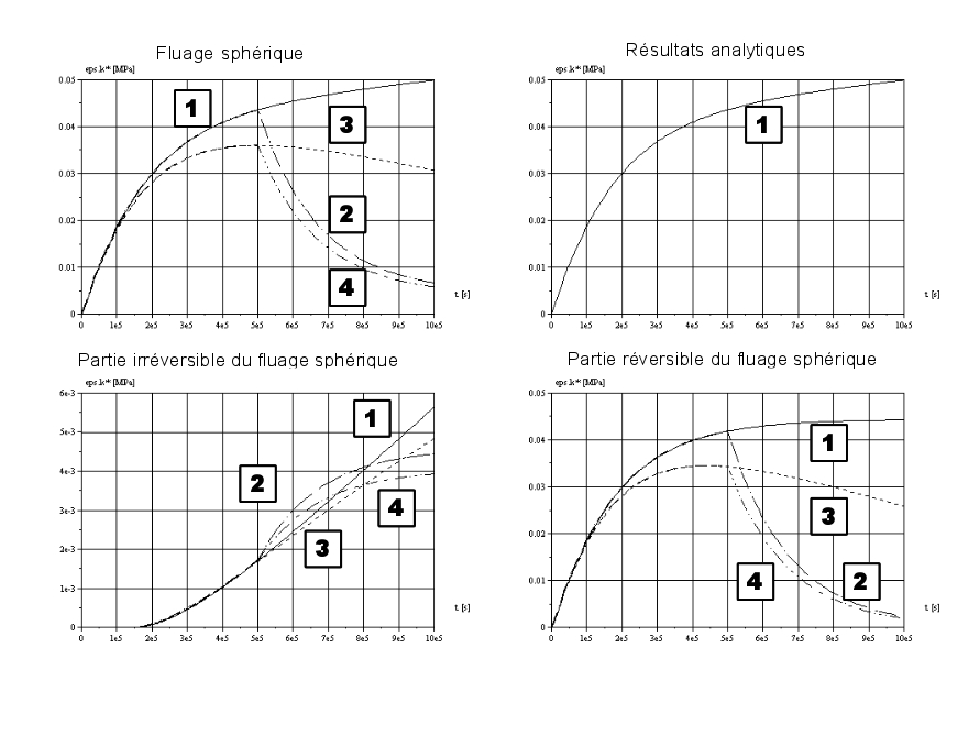
Figure 4.1-1: Numerical responses obtained using the discretized expressions [éq 4.1-3] to [éq4.1-17] for four loading stories: 1 unit stress step at constant humidity (100%), 2 unit stress step with linearly decreasing humidity from 100% to 50%, 3 unit stress step for half the duration of the calculation followed by a recovery of half of the initial stress on the second part of the calculation; humidity is assumed to be constant (100%)), 4 the mechanical loading is the same as 3; humidity decreases linearly from 100% to 50%.

To carry out the simulations of the the following parameters were selected: \({k}_{r}^{s}=\mathrm{2,0e+5}\) [MPa]; []; \({\eta }_{r}^{s}=\mathrm{4,0e}+\text{10}\) [MPa .s]; \({k}_{i}^{s}=\mathrm{1,0e+4}\) [MPa]; \({\eta }_{i}^{s}=\mathrm{1,0e}+\text{11}\) [MPa .s]. The calculation includes 200 intervals of 5000 [s].

4.2. Discretization of the equations constituting deviatoric creep

After discretizing the stresses and the relative humidity by affine functions, the deviating tensor of the natural creep deformations is discretized by the following equation:

\(\Delta {\underline{\underline{\epsilon }}}_{n}^{\text{fd}}={\underline{\underline{a}}}_{n}^{d}+{b}_{n}^{d}\cdot {\underline{\underline{\sigma }}}_{n}^{d}+{c}_{n}^{d}\cdot {\underline{\underline{\sigma }}}_{n+1}^{d}\) eq 4.2-1

where \({\underline{\underline{\sigma }}}_{n}^{d}\) and \({\underline{\underline{\sigma }}}_{n+1}^{d}\) are the deviatory stress tensors at the beginning and end of the current time step.

The steps carried out are:

The parameters are calculated in relation to the*reversible deviatoric natural creep deformation, whose model is:

\({\eta }_{r}^{d}{\underline{\underline{\dot{\epsilon }}}}_{r}^{\text{fd}}(t)+{k}_{r}^{d}{\underline{\underline{\epsilon }}}_{r}^{\text{fd}}(t)=h(t){\underline{\underline{\sigma }}}^{d}(t)\) eq 4.2-2

After discretization, the previous equation can be put in the form:

\(\Delta {\underline{\underline{\epsilon }}}_{r,n}^{\text{fd}}={\underline{\underline{a}}}_{r,n}^{d}+{b}_{r,n}^{d}\cdot {\underline{\underline{\sigma }}}_{n}^{d}+{c}_{r,n}^{d}\cdot {\underline{\underline{\sigma }}}_{n+1}^{d}\) eq 4.2-3

With:

\(\{\begin{array}{c}{\underline{\underline{a}}}_{r,n}^{d}=\left[\text{exp}(-\frac{{\mathrm{\Delta t}}_{n}}{{\tau }_{r}^{d}})-1\right]\cdot {\underline{\underline{\epsilon }}}_{r,n}^{f,d}\\ {b}_{r,n}^{d}=\frac{1}{{k}_{r}^{d}}\left\{\left[-(\frac{{\mathrm{2\tau }}_{r}^{d}}{{\mathrm{\Delta t}}_{n}}+1){h}_{n}+\frac{{\tau }_{r}^{d}}{{\mathrm{\Delta t}}_{n}}{h}_{n+1}\right]\text{exp}(-\frac{{\mathrm{\Delta t}}_{n}}{{\tau }_{r}^{d}})+\left[(\frac{{\mathrm{2\tau }}_{r}^{d}}{{\mathrm{\Delta t}}_{n}}-1){h}_{n}-\frac{{\tau }_{r}^{d}-{\mathrm{\Delta t}}_{n}}{{\mathrm{\Delta t}}_{n}}{h}_{n+1}\right]\right\}\\ {c}_{r,n}^{d}=\frac{1}{{k}_{r}^{d}}\left[\frac{{\tau }_{r}^{d}}{{\mathrm{\Delta t}}_{n}}\text{exp}(-\frac{{\mathrm{\Delta t}}_{n}}{{\tau }_{r}^{d}}){h}_{n}-\frac{{\tau }_{r}^{d}-{\mathrm{\Delta t}}_{n}}{{\mathrm{\Delta t}}_{n}}{h}_{n}\right]\end{array}\) eq 4.2-4

Note:

Equation [éq 4.2-4] (reversible part of deviatoric creep) is analogous to equation [éq4.1-5] (reversible part of creep in the absence of irreversible deformations). They correspond to the discretization of a single Kelvin chain.

The parameters are calculated with respect to the deviatoric natural creep deformation, whose model is:

\({\eta }_{i}^{d}{\underline{\underline{\dot{\epsilon }}}}_{i}^{f,d}(t)=h(t){\underline{\underline{\sigma }}}^{d}(t)\) eq 4.2-5

After discretization, the previous equation can be put in the form:

\(\Delta {\underline{\underline{\epsilon }}}_{i,n+1}^{f,d}={\underline{\underline{a}}}_{i,n}^{d}+{b}_{i,n}^{d}\cdot {\underline{\underline{\sigma }}}_{n}^{d}+{c}_{i,n}^{d}\cdot {\underline{\underline{\sigma }}}_{n+1}^{d}\) eq 4.2-6

With:

\(\{\begin{array}{c}{\underline{\underline{a}}}_{i,n}^{d}=0\\ {b}_{r,n}^{d}=\frac{{\mathrm{\Delta t}}_{n}\cdot {h}_{n+1}}{{\mathrm{2\eta }}_{i}^{d}}\\ {c}_{r,n}^{d}=\frac{{\mathrm{\Delta t}}_{n}\cdot {h}_{n}}{{\mathrm{2\eta }}_{i}^{d}}\end{array}\) eq 4.2-7

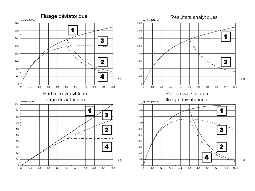
Figure 4.2-1: Numerical responses obtained using the discretized expressions [éq 4.2-1] to [éq4.2-7] for four loading stories: 1 unit stress step at constant humidity (100%), 2 unit stress step with linearly decreasing humidity from 100% to 50%, 3 unit stress step for half the duration of the calculation followed by recovery to half of the initial stress on the second part of the calculation; humidity is assumed to be constant (100%)), 4 the mechanical loading is the same as 3; humidity varies linearly decreasing from 100% to 50%.

To carry out the simulations of the, the following parameters were retained: \({k}_{r}^{d}=\mathrm{5,0e+4}\) [MPa]; []; \({\eta }_{r}^{d}=\mathrm{1,0e}+\text{10}\) [MPa .s]; \({\eta }_{i}^{d}=\mathrm{1,0e}+\text{11}\) [MPa .s]. The calculation includes 1000 intervals of 1000 [s].

4.3. Discretization of desiccation creep equations

The terms related to the consideration of desiccation creep are broken down according to the same concept as the terms of reversible proper creep [bib3]:

\(\Delta {\underline{\underline{\varepsilon }}}^{\mathit{fdess}}\mathrm{=}{\underline{\underline{a}}}_{n}^{\mathit{fdess}}+{b}_{n}^{\mathit{fdess}}\mathrm{\cdot }{\underline{\underline{\sigma }}}_{n}+{c}_{n}^{\mathit{fdess}}\mathrm{\cdot }{\underline{\underline{\sigma }}}_{n+1}\) eq. 4.3-1

The expression of the various terms is as follows:

\(\{\begin{array}{ccc}{\underline{\underline{a}}}_{n}^{\mathit{fdess}}& =& 0\\ {b}_{n}^{\mathit{fdess}}& =& \frac{\Delta {h}_{n}}{2\cdot {\eta }^{\mathit{fd}}}\\ {c}_{n}^{\mathit{fdess}}& =& \frac{\Delta {h}_{n}}{2\cdot {\eta }^{\mathit{fd}}}\end{array}\)