7. Coupling between BETON_UMLV and MAZARS#
Model BETON_UMLV is a model of linear viscoelastic behavior. To be able to represent the failure of concrete by tertiary creep, in Code_Aster, we propose to couple the creep model to a damage model, namely the MAZARS model (cf. [R7.01.08]). The coupling is carried out by assuming, on the one hand, that the creep deformations are generated by the effective stresses (i.e., those actually seen by the material) and on the other hand, that only a portion of the creep deformation (assumed to be constant) contributes to the evolution of the damage. The diagram is produced by maintaining the direct link between the state of elastic deformations and the state of stresses.
7.1. Implementation#
7.1.1. Updating internal variables for creep#
As for the rest of the document, we are limited here to the description of the coupling between damage and natural creep. We therefore assume as before that the deformation is written according to the equation [éq 2-2]:
\(\varepsilon ={\varepsilon }^{e}+{\varepsilon }^{f}\)
where \({\epsilon }^{e}\), elastic deformation, also contains the contribution of damage (micro-cracking) generated by the MAZARS model. By considering the spherical [éq 4.1-2] and deviatoric [éq 4.2-1] contributions of natural creep as well as that of desiccation creep, we obtain the increment of the creep deformations \(\Delta {\underline{\underline{\epsilon }}}^{f}\) between the times n and n+1:
\(\Delta {\underline{\underline{\varepsilon }}}_{n}^{f}={\underline{\underline{a}}}_{n}+{b}_{n}{\underline{\underline{\sigma }}}_{n}+{c}_{n}{\underline{\underline{\sigma }}}_{n+1}\) eq 6.1-1
with \({\underline{\underline{a}}}_{n},{b}_{n}{c}_{n}\) the total natural creep coefficients in linear viscoelasticity.
To introduce damage into the model, it is assumed that the creep deformations are generated by the effective stresses, noted \(\underline{\underline{\sigma }}\text{'}\) in the rest of the document. This allows delayed deformations to be associated with the integral part of the material, as proposed in [bib1].
It should be noted that the effective stresses can be written as a function of the damage variable \(D\) or (see also the documentation [R7.01.08-B]) as a law of elasticity:
\(\underline{\underline{\sigma }}\text{'}=\frac{\underline{\underline{\sigma }}}{1-D}=\underline{\underline{\underline{\underline{E}}}}{\underline{\underline{\varepsilon }}}^{e}\) eq 6.1-2
Therefore, equation [éq 6.1-1] becomes:
\(\Delta {\underline{\underline{\varepsilon }}}_{n}^{f}={\underline{\underline{a}}}_{n}+{b}_{n}\underline{\underline{\sigma }}{\text{'}}_{n}+{c}_{n}\underline{\underline{\sigma }}{\text{'}}_{n+1}\) eq 6.1-3
Using the law of elasticity [éq 6.1-2] with equation [éq 6.1-3], we obtain the new relationship for the creep deformation increment:
\(\Delta {\underline{\underline{\varepsilon }}}_{n}^{f}={(1+c\underline{\underline{\underline{\underline{E}}}})}^{\text{-1}}\left[{\underline{\underline{a}}}_{n}+{b}_{n}\underline{\underline{\sigma }}{\text{'}}_{n}+{c}_{n}\underline{\underline{\underline{\underline{E}}}}({\underline{\underline{\varepsilon }}}_{n+1}-{\underline{\underline{\varepsilon }}}_{n}^{f})\right]\) eq 6.1-4
Thus, from all the quantities known at time \(n\), it is possible to calculate with the relationship [éq 6.1-4] the creep deformation at time \(n+1\). Then, we easily obtain the effective constraints at time \(n+1\) thanks to the relationship [éq 6.1-2], and the internal variables of the creep with the equations [éq 4.1-2] and [éq 4.2-1].
7.1.2. Evolution of damage#
The MAZARS model is not detailed here; the reader may refer to the Code_Aster reference documentation for the MAZARS [R7.01.08] model.
The basic assumption is that damage is driven by elastic deformation and a share of creep deformation. The deformation tensor that drives the evolution of D is given by the following relationship:
\(\stackrel{˘}{\underline{\underline{\varepsilon }}}={\underline{\underline{\varepsilon }}}^{e}+\chi {\underline{\underline{\varepsilon }}}^{f}\) eq 6.2-1
with \(0\le \chi \le 1\) , coupling coefficient.
The coupling level is increasing with \(\chi\) increasing. So there are two edge cases: \(\chi =0\) and \(\chi =1\).
Yes, \(\chi =0\) there is an absence of coupling; the evolution of the damage depends only on the elastic deformation and therefore one cannot have tertiary creep.
If \(\chi =1\) the coupling is maximum, the damage depends on the total deformation. This case usually leads to premature ruin of the structure.
Note that the equation [éq 6.2-1] is equivalent to averaging the total and elastic deformations, using the \(\chi\) coefficient as the weight:
\(\stackrel{˘}{\underline{\underline{\varepsilon }}}=\chi \underline{\underline{\varepsilon }}+(1-\chi ){\underline{\underline{\varepsilon }}}^{e}\) eq 6.2-2a
or to subtract \(1-\chi\) times the creep deformations from the total deformations:
\(\stackrel{˘}{\underline{\underline{\varepsilon }}}=\underline{\underline{\varepsilon }}-(1-\chi ){\underline{\underline{\varepsilon }}}^{f}\) eq 6.2-2b
The equivalent deformation \({\epsilon }_{\mathit{eq}}\) that controls the damage in the coupled law is no longer evaluated from the elastic deformations but from the coupling deformations \(\stackrel{˘}{\underline{\underline{\varepsilon }}}\):
\({\varepsilon }_{\mathrm{eq}}=\sqrt{{\langle \stackrel{˘}{\underline{\underline{\varepsilon }}}\rangle }_{\text{+}}:{\langle \stackrel{˘}{\underline{\underline{\varepsilon }}}\rangle }_{\text{+}}}\) eq 6.2-3
\({\langle \rangle }_{\text{+}}\) corresponding to the positive part of the tensor.
The damage in tension \({D}_{t}\) and in compression \({D}_{c}\) are calculated as in the uncoupled case but with the equivalent deformation defined in equation [éq 6.2-3]:
\({D}_{c}=1-\frac{{\varepsilon }_{\mathrm{d0}}(1-{A}_{c})}{{\varepsilon }_{\mathrm{eq}}}-\frac{{A}_{c}}{\mathrm{exp}({B}_{c}({\varepsilon }_{\mathrm{eq}}-{\varepsilon }_{\mathrm{d0}}))}\) eq 6.2-4a
\({D}_{t}=1-\frac{{\varepsilon }_{\mathrm{d0}}(1-{A}_{t})}{{\varepsilon }_{\mathrm{eq}}}-\frac{{A}_{t}}{\mathrm{exp}({B}_{t}({\varepsilon }_{\mathrm{eq}}-{\varepsilon }_{\mathrm{d0}}))}\) eq 6.2-4b
( \({\varepsilon }_{\mathrm{d0}},{A}_{c},{B}_{c},{A}_{t},{B}_{t}\) ) being the material parameters of Mazars’s law.
As in the uncoupled case, a weighted average of these two damages by the coefficient
finally makes it possible to calculate the damage
:
eq 6.2-5a
eq 6.2-5b
Note that the choice that was made is to maintain the determination of the coefficient.
from the elastic deformations (and not the coupling deformations):
eq 6.2-6
where
are the natural deformations of the elastic tensor; the \({\varepsilon }_{\mathit{ti}}\) components of the tensor
are calculated from the eigenvalues of the elastic stresses
with the following elastic relationship:
eq 6.2-7
and
is the equivalent elastic deformation, calculated from the elastic deformation tensor
:
eq 6.2-8
Notes:
By adopting the elastic expression [éq 6.2-8], we find the conditions of the law of MAZARS: \({\alpha }_{t}=1\) for pure traction and \({\alpha }_{t}=0\) for pure compression.
There is a difference in the treatment of the dependence of Young’s modulus on temperature between the law of MAZARS and the law BETON_UMLV (keyword ELAS_FO of DEFI_MATERIAU). In the first case, the value of the module corresponding to the maximum temperature reached in the history of loading is used; in the second case, the user law is followed. In the case of coupling, this is the rule of law MAZARSqui is followed.
7.2. Traction response#
Here is an example of a response obtained with the coupled model. It is a bar with a variable cross section, locked at one end and with a tensile load applied to the free end.
In Figure 6.4-2, the damage map is shown at the end of the calculation for \(\chi \mathrm{=}1\); in Figure 6.4-1, the force-displacement response obtained for two values of \(\chi\) (1 and 0.9) is shown. The tertiary creep curve is well recognized, with the final rupture of the sample.
It is shown here that, under tension, the coupling coefficient mainly affects the breakage time.
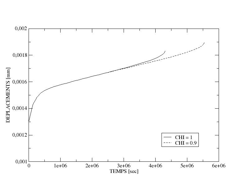
Figure 6.4-1: Tensile response on a bar for two values of the coupling coefficient.
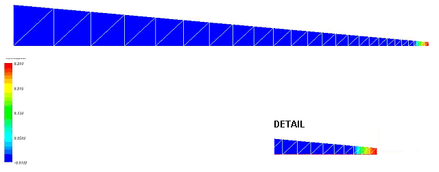
Figure 6.4-2: Damage to a bar where a tensile force has been applied ()
=1) .