3. Mixed variational formulation

Let’s transform the strong form of the problem into a weak formulation that is better suited to finite elements. Field \(u\) must belong to the \({V}_{0}\) set of kinematically eligible travel fields:

\({V}_{0}=\left\{v\in {H}^{1},v\text{discontinu}à\text{travers}{\Gamma }_{c},v=0\text{sur}{\Gamma }_{u}\right\}\)

Let’s start then by giving a unified formulation common to cases of touch-friction and regularized cohesive laws. Mixed cohesive laws in turn obey an energetic formulation following a different logic, explained in part 3.5.

3.1. Formalism common to regularized cohesive and to touch-friction

To do this we will note \(r\mathrm{=}{t}_{c}\) in the case of regularized laws. We note \(H\mathrm{=}{H}^{\mathrm{-}1\mathrm{/}2}(\Gamma )\) for cohesive laws, and we refer to \(H\) as the subspace of \({H}^{\mathrm{-}1\mathrm{/}2}(\Gamma )\) of contact action fields in the case of touch-friction. The weak formulation of the rubbing contact problem is written as follows:

Find \((u,{r}^{1},{r}^{2})\mathrm{\in }{V}_{0}\mathrm{\times }H\mathrm{\times }H\) such as:

\({\mathrm{\int }}_{\Omega }\sigma (u)\mathrm{:}\epsilon ({u}^{\text{*}})d\Omega \mathrm{=}{\mathrm{\int }}_{\Omega }f\mathrm{\cdot }{u}^{\text{*}}d\Omega +{\mathrm{\int }}_{{\Gamma }_{t}}t\mathrm{\cdot }{u}^{\text{*}}\mathit{d\Gamma }+{\mathrm{\int }}_{{\Gamma }^{1}}{r}^{1}\mathrm{\cdot }{u}^{{\text{*}}^{1}}{\mathit{d\Gamma }}^{1}+{\mathrm{\int }}_{{\Gamma }^{2}}{r}^{2}\mathrm{\cdot }{u}^{{\text{*}}^{2}}{\mathit{d\Gamma }}^{2}\mathrm{\forall }{u}^{\text{*}}\mathrm{\in }{V}_{0}\)

By writing the jump with the following notation

\([[x]]({P}^{1})=x({P}^{1})-x({P}^{2})\),

and noting \(r={r}^{1}\) and thereafter, the weak formulation of the rubbing contact problem is equivalently written as follows:

\({\mathrm{\int }}_{\Omega }\sigma (u)\mathrm{:}\varepsilon ({u}^{\text{*}})d\Omega \mathrm{=}{\mathrm{\int }}_{\Omega }f\mathrm{\cdot }{u}^{\text{*}}d\Omega +{\mathrm{\int }}_{{\Gamma }_{t}}t\mathrm{\cdot }{u}^{\text{*}}d\Gamma +{\mathrm{\int }}_{{\Gamma }_{c}}r\mathrm{\cdot }\mathrm{[}\mathrm{[}{u}^{\text{*}}\mathrm{]}\mathrm{]}d{\Gamma }_{c}\mathrm{\forall }{u}^{\text{*}}\mathrm{\in }{V}_{0}\)

The contact unknowns spaces are as follows:

\(\begin{array}{c}H\mathrm{=}\left\{\lambda \mathrm{\in }{H}^{\mathrm{-}1\mathrm{/}2}({\Gamma }_{c}),\lambda \mathrm{\le }0\text{sur}{\Gamma }_{c}\right\}\\ H\mathrm{=}\left\{{r}_{\tau }\mathrm{\in }{H}^{\mathrm{-}1\mathrm{/}2}({\Gamma }_{c}),\mathrm{\parallel }{r}_{\tau }\mathrm{\parallel }\mathrm{\le }\mu \lambda \text{sur}{\Gamma }_{c}\right\}\end{array}\)

3.2. Augmented Lagrangian method

The weak formulation with three fields is finally written, in the case of an augmented Lagrangian formation:

Find \((u,\lambda ,\Lambda )\in {V}_{0}\times H\times H\)

\(\forall ({u}^{\text{*}},{\lambda }^{\text{*}},{\Lambda }^{\text{*}})\in {V}_{0}\times H\times H\)

Equation of balance	\(\begin{array}{c}{\mathrm{\int }}_{\Omega }\sigma (u)\mathrm{:}\epsilon ({u}^{\text{*}})d\Omega \mathrm{-}{\mathrm{\int }}_{\Omega }f\mathrm{\cdot }{u}^{\text{*}}d\Omega \mathrm{-}{\mathrm{\int }}_{{\Gamma }_{t}}t\mathrm{\cdot }{u}^{\text{*}}\mathit{d\Gamma }\\ \mathrm{-}{\mathrm{\int }}_{{\Gamma }_{c}}\chi ({g}_{n}){g}_{n}n\mathrm{\cdot }\mathrm{[}\mathrm{[}{u}^{\text{*}}\mathrm{]}\mathrm{]}{\mathit{d\Gamma }}_{c}\mathrm{-}{\mathrm{\int }}_{{\Gamma }_{c}}\chi ({g}_{n}){\text{μλ}}_{s}{{\rm P}}_{{\rm B}(\mathrm{0,1})}({g}_{\tau })\mathrm{\cdot }\mathrm{[}\mathrm{[}{u}_{\tau }^{\text{*}}\mathrm{]}\mathrm{]}{\mathit{d\Gamma }}_{c}\mathrm{=}0\end{array}\)
Law of contact	\({\mathrm{\int }}_{\mathit{\Gamma c}}\frac{\mathrm{-}1}{{\rho }_{n}}(\lambda \mathrm{-}\chi ({g}_{n}){g}_{n}){\lambda }^{\text{*}}{\mathit{d\Gamma }}_{c}\mathrm{=}0\)
Law of friction	\(\begin{array}{c}{\mathrm{\int }}_{\mathit{\Gamma c}}\frac{\text{μχ}({g}_{n}){\lambda }_{s}\mathit{\Delta t}}{{\rho }_{\tau }}(\Lambda \mathrm{-}{P}_{B(\mathrm{0,1})}({g}_{\tau })){\Lambda }^{\text{*}}{\mathit{d\Gamma }}_{c}\\ +{\mathrm{\int }}_{\mathit{\Gamma c}}(1\mathrm{-}\chi ({g}_{n}))\Lambda {\Lambda }^{\text{*}}{\mathit{d\Gamma }}_{c}\mathrm{=}0\end{array}\)

3.3. Penalized method

The weak formulation with three fields is finally written, in the case of purely penalized training:

Find \((u,\lambda ,\Lambda )\mathrm{\in }{V}_{0}\mathrm{\times }H\mathrm{\times }H\)

\(\mathrm{\forall }({u}^{\text{*}},{\lambda }^{\text{*}},{\Lambda }^{\text{*}})\mathrm{\in }{V}_{0}\mathrm{\times }H\mathrm{\times }H\)

Equation of balance	\(\begin{array}{c}{\mathrm{\int }}_{\Omega }\sigma (u)\mathrm{:}\epsilon ({u}^{\text{*}})d\Omega \mathrm{-}{\mathrm{\int }}_{\Omega }f\mathrm{\cdot }{u}^{\text{*}}d\Omega \mathrm{-}{\mathrm{\int }}_{{\Gamma }_{t}}t\mathrm{\cdot }{u}^{\text{*}}\mathit{d\Gamma }\\ \mathrm{-}{\mathrm{\int }}_{{\Gamma }_{c}}\chi ({g}_{n})\lambda \mathrm{\cdot }\mathrm{[}\mathrm{[}{u}^{\text{*}}\mathrm{]}\mathrm{]}\mathrm{\cdot }n{\mathit{d\Gamma }}_{c}\\ \mathrm{-}{\mathrm{\int }}_{{\Gamma }_{c}}\chi ({g}_{n}){\text{μλ}}_{s}{{\rm P}}_{{\rm B}(\mathrm{0,1})}({\kappa }_{\tau }{\nu }_{\tau })\mathrm{\cdot }\mathrm{[}\mathrm{[}{u}_{\tau }^{\text{*}}\mathrm{]}\mathrm{]}{\mathit{d\Gamma }}_{c}\mathrm{=}0\end{array}\)
Law of contact	\({\mathrm{\int }}_{\mathit{\Gamma c}}\frac{\mathrm{-}1}{{\kappa }_{n}}(\lambda +\chi ({g}_{n}){\kappa }_{n}{d}_{n}){\lambda }^{\text{*}}{\mathit{d\Gamma }}_{c}\mathrm{=}0\)
Law of friction	\(\begin{array}{c}{\mathrm{\int }}_{\mathit{\Gamma c}}\frac{\text{μχ}({g}_{n}){\lambda }_{s}}{{\kappa }_{\tau }}(\Lambda \mathrm{-}{P}_{B(\mathrm{0,1})}({\kappa }_{\tau }{\nu }_{\tau })){\Lambda }^{\text{*}}{\mathit{d\Gamma }}_{c}\\ +{\mathrm{\int }}_{\mathit{\Gamma c}}(1\mathrm{-}\chi ({g}_{n}))\Lambda {\Lambda }^{\text{*}}{\mathit{d\Gamma }}_{c}\mathrm{=}0\end{array}\)

Note that the value of \(\lambda\) obtained by the law of contact is an average when the state is contacting interpenetrating forces for the penalized law. The use of the expressions \(\lambda\) or \(-{\kappa }_{n}{d}_{n}\) in the balance equation should therefore lead to the same result except that the condition LBB only applies to the \(\lambda\). To have equivalence, it would therefore be necessary to postpone the treatment of LBB to the displacement fields for the penalized method. As this is not done here, we use the term \(\lambda\) for which the LBB treatment is done and we reinject it into the equilibrium equation which therefore takes this treatment into account. We could try the same treatment for the law of friction but \(\Lambda\) is obtained as an average for slippery or adherent situations. Reinjecting this averaged state into the equilibrium equation leads to a non-convergence of Newton’s algorithm. The difference in behavior for \(\lambda\) and \(\Lambda\) comes from the fact that we integrate discontinuous quantities according to the contacting or non-contacting state for \(\lambda\) and according to the sliding or adherent state for \(\Lambda\), but that for the non-contacting state the contributions on \(\lambda\) are zero in the contact law. It can be deduced from this that while there is a penalized formulation fully satisfying conditions LBB for contact, for the moment there is no penalized formulation fully satisfying conditions LBB for friction. The choice of the \({\kappa }_{\tau }\) coefficient will therefore be all the more important (high values may present obstacles for the adhering party).

3.4. Formulation for a cohesive regularized law

When a cohesive law is used, contact is managed by the penalty coefficient defined in the cohesive law. Knowing the expression of cohesive law in terms of \(\mathrm{〚}u\mathrm{〛}\), the formulation is written:

Find \((u,\lambda ,\Lambda )\in {V}_{0}\times H\times H\) such as:

\(\forall ({u}^{\text{*}},{\lambda }^{\text{*}},{\Lambda }^{\text{*}})\in {V}_{0}\times H\times H\)

Equation of balance	:math:`begin{array}{c}{mathrm{int }}_{Omega }sigma (u)mathrm{:}epsilon ({u}^{text{*}})dOmega mathrm{-}{mathrm{int }}_{Omega }fmathrm{cdot }{u}^{text{*}}dOmega mathrm{-}{mathrm{int }}_{{Gamma }_{t}}tmathrm{cdot }{u}^{text{*}}mathit{dGamma }\ mathrm{-}{mathrm{int }}_{{Gamma }_{c}}{t}_{c	n}mathrm{cdot }{mathrm{〚}{u}^{text{*}}mathrm{〛}}_{n}{mathit{dGamma }}_{c}mathrm{-}{mathrm{int }}_{{Gamma }_{c}}{t}_{c	tau }mathrm{cdot }{mathrm{〚}{u}^{text{*}}mathrm{〛}}_{tau }{mathit{dGamma }}_{c}mathrm{=}0end{array}`
Post-treatment normal part	:math:`{mathrm{int }}_{mathit{Gamma c}}(lambda mathrm{-}{t}_{c	n}mathrm{cdot }n){lambda }^{text{*}}{mathit{dGamma }}_{c}mathrm{=}0`
Post-processing tangential part	:math:`{mathrm{int }}_{mathit{Gamma c}}(Lambda mathrm{-}{t}_{c	tau }){Lambda }^{text{*}}{mathit{dGamma }}_{c}mathrm{=}0`

Note that the multipliers \(\lambda\) and \(\Lambda\) are not involved in the resolution. They are only used to store cohesive constraints explicitly.

3.5. Formulation for a cohesive mixed law

In contrast to the previous formulation, the treatment of such a law will require a real formulation with several fields, in the sense that a dual vector field \(\lambda\) will actually enter the formulation, instead of being a post-processing device as in 3.4. This formulation follows energetic reasoning, explained in detail in the documentation [R3.06.13]. Let’s summarize the main points:

We write that the opening of the crack costs an energy proportional to the area to be opened, i.e.:

\({E}_{\text{fr}}(\delta )\mathrm{=}\underset{\Gamma }{\mathrm{\int }}\Pi (\delta )\text{dS}\)

where \(\Pi (\delta )\) is the cohesive energy density. For law CZM_OUV_MIX, for example, we have \(\Pi (\delta )\mathrm{=}{\mathrm{\int }}_{0}^{{\delta }_{n}}{t}_{c,n}(\delta \text{'})d\delta \text{'}\).

The discontinuity field \(\delta\) appearing in the previous expressions is then defined as a field in its own right, integrated into the formulation as a new unknown. The total energy is then written as:

\(E(u,\delta )\mathrm{=}\underset{\Omega \mathrm{\setminus }\Gamma }{\mathrm{\int }}\Phi (\epsilon (u))d\Omega \mathrm{-}{W}_{\mathit{ext}}(u)+\underset{\Gamma }{\mathrm{\int }}\Pi (\delta )\mathit{d\Gamma }\)

The solution of the problem then consists in minimizing this total energy under the constraint that \(\delta\) corresponds, with our sign conventions, to the opposite of the displacement jump. We are looking for:

\(\underset{\begin{array}{c}u,\delta \\ \left[\left[u\right]\right]\mathrm{=}\mathrm{-}\delta \end{array}}{\text{min}}E(u,\delta )\)

In order to solve this problem, we introduce the Lagrangian associated with the problem, to which we add an augmentation term whose usefulness will appear later:

\({L}_{r}(u,\delta ,\lambda )\underset{\mathit{déf.}}{\mathrm{=}}E(u,\delta )+\underset{\Gamma }{\mathrm{\int }}\lambda \mathrm{\cdot }(\mathrm{-}\mathrm{〚}u\mathrm{〛}\mathrm{-}\delta )\mathit{d\Gamma }+\underset{\Gamma }{\mathrm{\int }}\frac{r}{2}{(\mathrm{〚}u\mathrm{〛}+\delta )}^{2}\mathit{d\Gamma }\)

We can then write the first optimality condition for this Lagrangian:

\(\mathrm{\forall }{\delta }^{\text{*}}\underset{\Gamma }{\mathrm{\int }}\left[t\mathrm{-}\lambda +r(\mathrm{〚}u\mathrm{〛}+\delta )\right]\mathrm{\cdot }{\delta }^{\text{*}}\mathrm{=}0\text{avec}t\mathrm{\in }\mathrm{\partial }\Pi (\delta )\)

This equation involves the cohesive constraint \({t}_{c}\). However, we only have a local law of behavior as an expression of \({t}_{c}\). This first equation must therefore, in order to make sense, be discretized in a way that makes it possible to reduce it to a local expression. This is possible if \(\delta\) is discretized by collocation at the Gauss points of the interface, with coordinates \({x}_{g}\).

In fact, with such discretization, resolving the first optimality condition amounts to satisfying the cohesive law at each collocation point:

\({t}_{c}({\delta }_{g},{\alpha }_{g})\mathrm{=}{\lambda }_{g}\mathrm{-}r(\mathrm{〚}{u}_{g}\mathrm{〛}+{\delta }_{g})\)

where we noted \({\lambda }_{g}\mathrm{=}\lambda ({x}_{g})\), for example, the values of a field at Gauss points, and where \({t}_{c}({\delta }_{g},{\alpha }_{g})\) follows the law. The graphical translation of this law of behavior is as follows: the solution corresponds to the intersection of the linear function \(\delta \to {\lambda }_{g}\mathrm{-}r\mathrm{〚}{u}_{g}\mathrm{〛}\mathrm{-}r\delta\) (with a negative slope given by the penalty coefficient \(r\)) with the graph \({t}_{c}(\delta ,\alpha )\). We then see that for \(r\) that is quite large, the solution is unique, which is why it is interesting to have increased the Lagrangian.

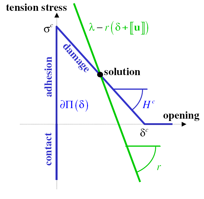
Figure 3.5-a: Behavioral integration solution.

Field \(\delta\) is therefore written locally as a function of \(\lambda \mathrm{-}r\mathrm{〚}u\mathrm{〛}\), which we will call an increased multiplier and write it down as \(p\). As a result, unknown fields of the problem disappear. The formulation is then given by the two remaining Lagrangian optimality conditions:

Find \((u,\lambda )\mathrm{\in }{V}_{0}\mathrm{\times }H\) such as:

\(\mathrm{\forall }({u}^{\text{*}},{\lambda }^{\text{*}})\mathrm{\in }{V}_{0}\mathrm{\times }H\)

.csv-table:

Equation of balance, \(\begin{array}{c}{\mathrm{\int }}_{\Omega }\sigma (u)\mathrm{:}\epsilon ({u}^{\text{*}})d\Omega \mathrm{-}{\mathrm{\int }}_{\Omega }f\mathrm{\cdot }{u}^{\text{*}}d\Omega \mathrm{-}{\mathrm{\int }}_{{\Gamma }_{t}}t\mathrm{\cdot }{u}^{\text{*}}d\Gamma \\ +{\mathrm{\int }}_{{\Gamma }_{c}}\left[\mathrm{-}\lambda +r(\mathrm{〚}u\mathrm{〛}+\delta (p))\right]\mathrm{\cdot }\mathrm{〚}{u}^{\text{*}}\mathrm{〛}d\Gamma \mathrm{=}0\text{avec}p\mathrm{=}\lambda \mathrm{-}r\mathrm{〚}u\mathrm{〛}\end{array}\) Interface law, \(\mathrm{-}{\mathrm{\int }}_{{\Gamma }_{c}}\left[\mathrm{〚}u\mathrm{〛}+\delta (p)\right]\mathrm{\cdot }{\lambda }^{\text{*}}d\Gamma \mathrm{=}0\)

With regard to the discretization of these two fields of unknowns, a simple discretization respecting the stability condition inf-sup, and consistent with the discretization of \(\delta\) by collocation, consists in discretizing the displacement with elements P 2 and the multiplier in a way P1 adapted to X- FEM, which we will give details of in part 4.1 to follow.