4. EF discretizations#
In this part, we detail the discretization of the contact/friction unknowns, which takes place at the top nodes of the parent element.
4.1. Contact multipliers#
The unknowns for contact pressure \(\lambda\) and the friction semi-multiplier \(\Lambda\) are taken to the vertex nodes of the parent element. The approximation of the contact pressure involves the \({\phi }_{i}\), a function of the shape of the linear parent element and is written as:
\({\lambda }^{h}(x)=\sum _{i=1}^{\mathrm{nno}}{\lambda }_{i}{\phi }_{i}(x)\)
where \(\mathrm{nno}\) is the number of nodes in the linear parent element. The pressure is then defined as the trace on the interface approximated to this field \({\lambda }^{h}\).
To explain this concept of an approximate interface, let’s assume that we cut, if necessary, the parent element into simplicial sub-elements (i.e. triangles in 2D, tetrahedra in 3D). By approximate interface, in 2D, we mean the broken line connecting together the intersection points of the edges of such sub-elements with the crack line. In 3D, the points of intersection of the edges of such a sub-element with the surface of the crack define a polygon, which is not necessarily plane within this sub-element: for example, there may be 4 intersection points, not necessarily coplanar. The method chosen was that which consisted in cutting this polygon into triangular facets whose vertices are these intersection points ([fig.]). The entire method described in this paragraph is detailed in part 4.3.
4.2. Friction semi-multipliers#
As with contact multipliers, friction semi-multipliers are interpolated with the \({\phi }_{i}\) shape function of the parent element. In 3D, \(\Lambda\) is a vector from the tangential plane to the surface of the crack. The gradients of the level sets make it possible to define a covariant base at the surface of the crack, in which \(\Lambda\) will be expressed. The 2 vectors of the covariant base are defined by:
\(({n}^{\mathrm{ls}},{\tau }^{1},{\tau }^{2})=(\nabla \mathrm{lsn},\nabla \mathrm{lst},\nabla \mathrm{lsn}\times \nabla \mathrm{lst})\)
where \({n}^{\mathrm{ls}}\) is the local normal from the normal level-set gradient. Since the vectors \({\tau }^{1},{\tau }^{2}\) come from the (nodal) gradients of the level sets, they can be interpolated within the elements in order to obtain vectors at the vertices \(i\) of the contact facets, i.e. \({\tau }_{i}^{1}\) and \({\tau }_{i}^{2}\), \(i=\mathrm{1,3}\). The approximation of the friction semi-multipliers on a contact facet is then written:
\({\Lambda }^{h}(x)=\sum _{i=1}^{\mathrm{nno}}({\Lambda }_{i}^{1}{\tau }_{i}^{1}+{\Lambda }_{i}^{2}{\tau }_{i}^{2}){\phi }_{i}(x)\),
where the vectors \({\tau }_{i}^{1},{\tau }_{i}^{2}\) for a node i correspond to those of the intersection point of the interface with the edge of the element associated with node i. The associated intersection point is either this node (if it is a node through which the contact interface passes) or the intersected edge containing this node (if it is a cut edge). In the case where the node belongs to several intersecting edges, it is associated with the point of intersection of the vital edge.
4.3. Finite contact element#
4.3.1. General case#
The contact degrees of freedom are carried exclusively by the vertex nodes.
As an example, the figure shows the knots carrying the contact degrees of freedom. Note that one distinguishes on the one hand the X- FEM elements cut by the crack which will carry contact degrees of freedom and on the other hand the uncut X- FEM elements which do not need contact degrees of freedom. Contact degrees of freedom are introduced only on the vertex nodes, i.e. a total of 4 degrees of freedom. Two equality relationships connect nodes 1 and 3 as well as nodes 2 and 4 respectively in order to satisfy condition LBB (see [§ 6]). This makes a total of 6 variables introduced.
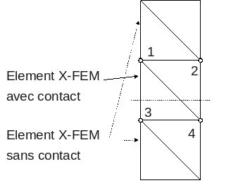
Figure 4.3.1-1 : Nodes carrying contact ddls.
FACETTE OF CONTACT
The contact surface is only used for integration purposes but it requires the establishment of an algorithm for finding intersection points and midpoints if the element is quadratic.
The algorithm for finding intersection points is as follows:
On an element:
loop over the edges of the element
Let \({E}^{1}\) and \({E}^{2}\) be the two ends of the edge
If \(\text{lsn}({E}^{1})\text{lsn}({E}^{2})\le 0\) then
buckle on both ends
If \(\text{lsn}({E}^{j})=0\) and \(\text{lst}({E}^{j})\le 0\) then
we add the point \({E}^{j}\) to the list of \({P}_{i}\) (with verification of duplicates)
Ending yes
if 2D quadratic element: \(\text{lsn}({E}^{3})=0\) and \(\text{lst}({E}^{3})\le 0\) then
we add the point \({E}^{3}\) to the list of \({P}_{i}\) (with verification of duplicates)
Ending yes
end loop
if \(\text{lsn}({E}^{k})\ne 0\forall k\in\) number of nodes on the edge, then
C coordinate interpolation
If \(\text{lst}(C)\le 0\) then
we add the point \(C\) to the list of \({P}_{i}\) (with verification of duplicates)
Ending yes
Ending yes
Ending yes
end loop
Details of the interpolation of the coordinates of point C:
If the element is linear:
\(s=\frac{\text{lsn}({E}^{1})}{\text{lsn}({E}^{1})-\text{lsn}({E}^{2})}\)
\(C={E}^{1}-s({E}^{2}-{E}^{1})\)
\(\text{lst}(C)=\text{lst}({E}^{1})-s(\text{lst}({E}^{2})-\text{lst}({E}^{1}))\)
If the element is 2D quadratic:
The position of the point on the edge provides information on the value of one of its reference coordinates \(\xi\) or \(\eta\), it is then sufficient to solve the polynomial equation \(\sum _{i=1}^{\mathrm{nno}}{\Phi }_{i}(\xi ,\eta ){\mathrm{lsn}}_{i}=0\) to find the value of the second reference coordinate. By passing through the real element, we determine its real coordinates \((x,y)\).
Ending yes
In the case where the element is quadratic, in addition to the intersection points, it is necessary to interpolate the coordinates of the middle nodes of the contact facet. In 2D, the contact facet is similar to an arc where we only know the coordinates of its ends following the previous algorithm. To determine its midpoint, we use Newton’s method, which evaluates the intersection point between the mediator of the segment connecting the two ends and the izo-zero of the normal level set.
4.3.2. Case of elements at the bottom of a crack#
For an element containing the bottom of the crack, special treatment is required to determine the contact points. In fact, such elements are not entirely cut by the crack. The contact points are then of two types:
or intersections between the surface of the crack and the edges of the element (general case mentioned in the previous paragraph),
or intersections between the crack bottom and the faces of the element (case specific to elements containing the crack bottom).
The points of the 1st type are determined by the previous algorithm, and the points of the 2nd type by the algorithm for finding points at the bottom of the crack (see paragraph [§2.4] in [R7.02.12]).
The contact points of the 2nd type are not associated with any node or edge, and are therefore not carried natively by any ddl. They are therefore not involved in writing the approximation. This situation corresponds to an approximation P1 of the contact unknowns on the contact facet at the bottom, having a zero value at the bottom of the crack (see diagram at the top of Figure 4.3.2-1). Another solution is to consider a constant connection. In this case, the pressure at the bottom of the crack is considered equal to the pressure of the contact point on a nearest edge. It was this solution that was adopted. In the example in Figure 4.3.2-1, the diagram at the bottom illustrates the approximation of the contact pressure on facet \(\text{ABC}\):
\(\begin{array}{ccc}\lambda (x)& \text{=}& {\lambda }_{A}{\psi }_{A}+{\lambda }_{B}{\psi }_{B}+{\lambda }_{C}{\psi }_{C}\\ & \text{=}& {\lambda }_{D}{\psi }_{A}+{\lambda }_{C}{\psi }_{B}+{\lambda }_{C}{\psi }_{C}\end{array}\)
Since \(\text{BC}<\text{BD}\) and \(\text{AD}<\text{AC}\), the pressure unknown in \(B\) is carried by the point \(C\) and the pressure unknown in \(A\) is carried by the point \(D\), so there is no additional ddl on the faces. This approach could be referred to as « P0-P1 » because the approximation is a mixture of P0 and P1. The contact pressure is P1 along the crack bottom, and P0 along the other sides of the facet.
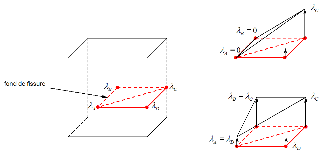
Figure 4.3.2-1 : Different approximations of contact on the facet at the bottom of the crack
Another alternative would be to consider a true approximation P1 on the contact facets at the bottom of the crack. To do this, the degrees of freedom of contact on the background points would have to be true independent degrees of freedom. For example, they could be carried by the node vertices of opposite edges. On the example of Figure 4.3.2-2, the contact pressure in \(B\) would be carried by the node \(F\) and the contact pressure in \(A\) by the node \(E\). This case can be generalized to any type of configuration. The advantage is to have degrees of freedom of independent contact. Such an approximation P1 would improve the precision compared to a constant approximation.
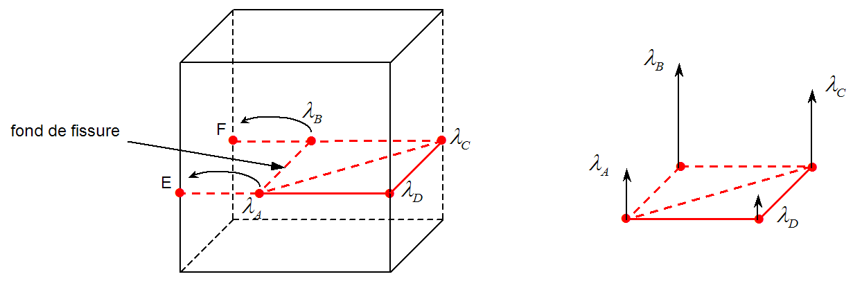
Figure 4.3.2-2 : Approximation P1 on the contact facet at the bottom of the crack
4.3.3. Sub-division into triangular contact facets#
For each element, based on the list of contact points \({P}_{i}\), a sub-division into triangular facets must be created. To do this, the contact points are sorted by element using the same process as that used to orient the points of the crack bottom (see paragraph [§2.4] in [R7.02.12]). We determine \(n\) the mean of the normals at the nodes (based on the gradients of the level sets). We determine \(G\) the barycenter of the contact points on this element. The contact points are projected into the plane of normal \(n\) and going through \(G\). For each of the projected ones, we determine the angle \(\theta\) in relation to the 1st point in the list, then we sort the points in the list as \(\theta\) ascending.
To illustrate the sub-division into triangular facets, let’s take a hexahedron occupying region \({\left[\mathrm{0,1}\right]}^{3}\). Consider the Cartesian equation plane \(\mathrm{4x}-\text{11}y-\mathrm{9z}+d=0\). Let’s look at the intersections between this plane and the hexahedron, for various values of the \(d\) parameter.
For \(d=-1\), there are 3 intersection points between the plane and the hexahedron. The outline of the plane in the hexahedron is a triangle, which corresponds to the contact facet. For \(d=4\), there are 4 intersection points between the plane and the hexahedron. The trace of the plane in the hexahedron is a quadrangle, is divided into two triangular contact facets. For \(d=6\), there are 5 intersection points between the plane and the hexahedron. The trace of the plane in the hexahedron is a pentagon, is divided into three triangular contact facets. For \(d\mathrm{=}8\), there are 6 intersection points between the plane and the hexahedron. The plane trace in the hexahedron is a hexagon, is cut into four triangular contact facets. Figure 4.3.3-1 shows the various patterns for the \(d\) values mentioned above.
In addition, when the crack bottom is contained in an element, it may add an additional intersection point. For example for \(d=8\), if the crack bottom intersects the segments P1P2 and P2P3 then this adds a point P2a located on P1P2 and another point P2b located on P2 P3 and removes the point P2 (2 points added and 1 point removed, i.e. in total 1 point added). The maximum number of intersection points is then 7.
This example illustrates the various scenarios that can occur. In general, the various scenarios can be grouped together according to the number of intersection points encountered. Tableau 4.3.3-1 brings together the sub-cuts made according to the number of intersection points found between the element (whether the element is a tetrahedron, pentahedron, or hexahedron) and the surface of the crack.
3 intersection points |
4 intersection points |
5 intersection points |
6 intersection points |
7 intersection points |
|
Triangular facets |
P1 P2 P3 |
P1 P2 P3 |
P1 P2 P3 |
||
P1 P3 P4 » |
P1 P2 P3 P1 P3 P4 P1 P4 P5 |
P1 P2 P3 P1 P3 P5 P1 P5 P6 P3 P4 P5 |
P1 P2 P3 P1 P3 P5 P3 P4 P5 P1 P5 P7 P5 P6 P7 |
Table 4.3.3-1 : Triangular facet breaking
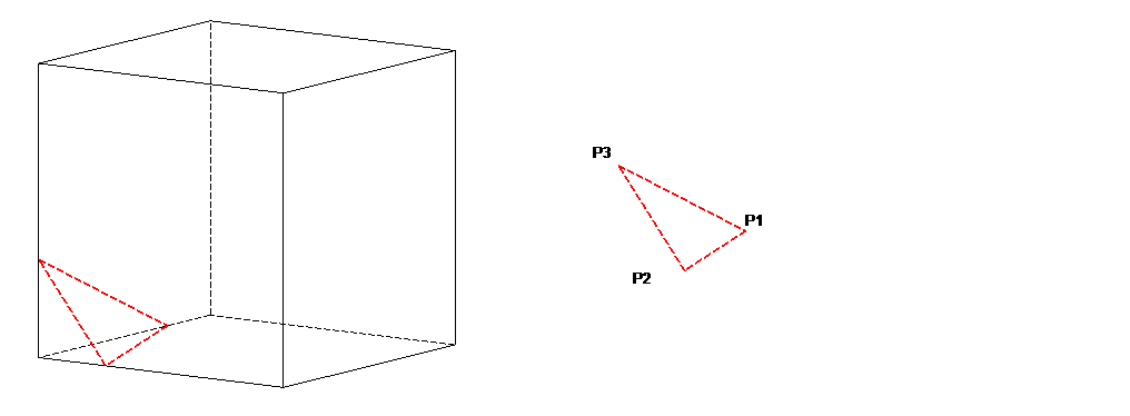
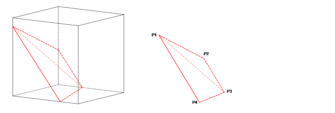
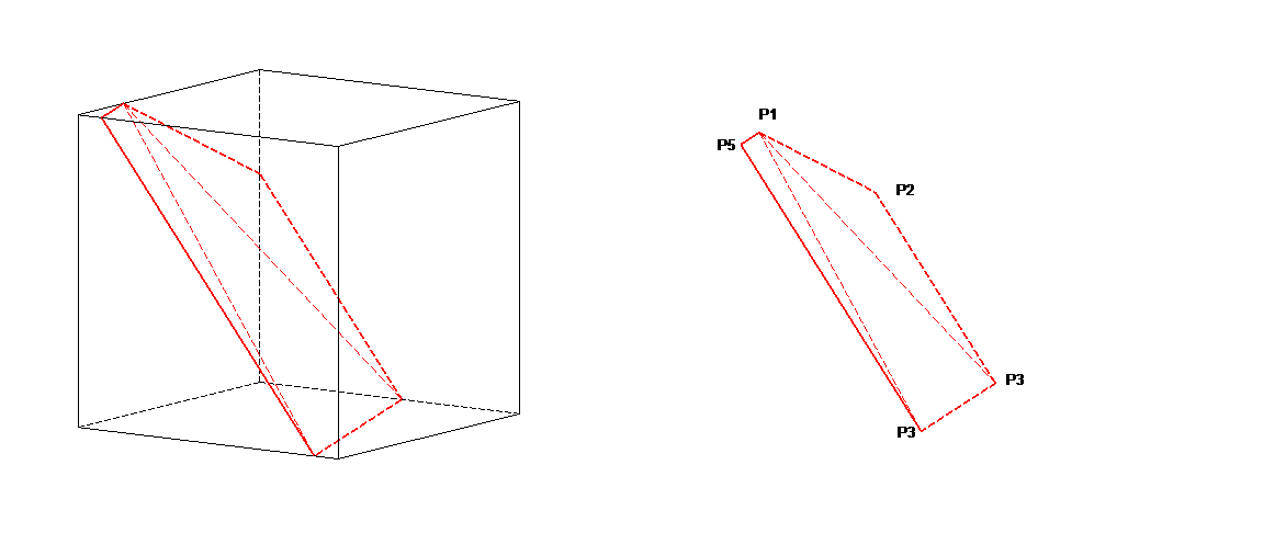
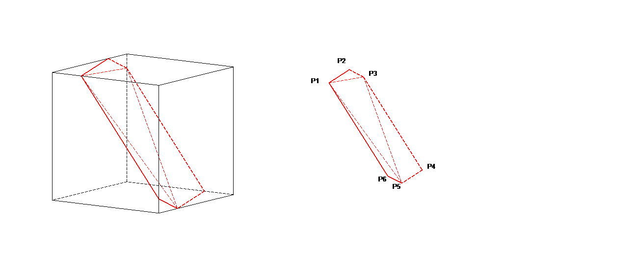
Figure 4.3.3-1 : Intersections and cuts for d = -1, 4, 6, and 8 (top to bottom)
4.4. Setting inactive degrees of freedom to zero#
This procedure is used to zero the value of the degrees of freedom of which are not involved in the equations. Several solutions can be considered.
Note:
The following discussion is strongly influenced by the possibilities (and limitations) of Code_Aster; the solutions considered cannot therefore be exhaustive.
4.4.1. Do not introduce#
First of all, couldn’t we simply avoid introducing these degrees of freedom that are useless and that will have to be canceled later? For example, one could imagine an element initially without a contact degree of freedom, and once the intersections between the edges of the element and the crack have been determined, add the necessary degrees of contact freedom. This would mean transforming the finite element into a finite element with contact degrees of freedom in certain specific nodes (for example at nodes \(\mathit{N1}\), \(B\), \(C\), \(\mathit{N4}\) in fig.). It is easy to see the number of possibilities this represents, and the number of different finite elements that this would involve (21 for a tetrahedron with 3 or 4 points of intersection, and more than 150 for a hexahedron with 3, 4, 5 or 6 points of intersection). This solution is therefore rejected. It is therefore necessary to have a contact element with contact degrees of freedom on all the vertex and middle nodes.
4.4.2. Elimination#
To eliminate the useless degrees of contact freedom, the simplest idea is to remove the corresponding rows and columns from the overall system of equations (on paper, this is the same as « crossing out » useless rows and columns). The system obtained is therefore smaller in size than the total system, and of the same size as that which would have been obtained with the method in the preceding paragraph. However, removing rows and columns from the global system is currently not possible in Code_Aster.
4.4.3. Substitution#
If you cannot eliminate degrees of freedom, you must assign them the value 0. To do this, we can decide to modify the tangent matrix and the second member, by putting any real value \({k}_{0}\) (for example 1) on the diagonal of the matrix and 0 in the second member, at the position corresponding to the degree of freedom to be canceled. We therefore have a system of the same size, but numerically poorly conditioned because of any value chosen on the diagonal. In fact, at the level of calculating the elementary matrix, the stiffness matrix is not known globally, so the optimal value of the parameter \({k}_{0}\) (in terms of conditioning) is not known.
4.4.4. Dualization#
To overcome this kind of problem, the DDL_IMPO keyword of the AFFE_CHAR_MECA operator makes it possible to impose a predefined value on a node’s degree of freedom. To solve the linear system under constraints thus obtained, the Lagrange double multipliers technique is used [bib 5], which allows better conditioning than with the simplistic technique in the previous paragraph, because the choice of the parameters \({k}_{0}\) is made knowing the assembled matrix. The main disadvantage is that two additional equations are added to the system for each ddl imposed.
4.4.5. Generalized substitution#
The substitution method is generalized to the imposition of ddl at any value (other than 0) in Code_Aster (operator AFFE_CHAR_CINE). However, this operator does not currently work with the nonlinear static operator (STAT_NON_LINE) used to solve the system (the non-linearity of the problem treated is due to touch-friction).
4.4.6. Solution selected#
The removal is useful for bilinear meshes and crack bottoms. This is done using the substitution method: however, this choice must be monitored, or even studied more closely, in terms of robustness, as there are possible impacts on the stability of convergence. For the rest, namely relationships of equality, the solution that was adopted was that of double Lagrange multipliers. Note that with the use of Mumps as a solver, only one multiplier is taken into account. However, we realized that the argument about poor conditioning that led us to not choose the substitution method does not hold up. Of course, the matrix may be poorly conditioned, but this has no impact on the quality of the results since the matrix is block by block (for example, the \(\mathit{diag}(1,10.e16)\) diagonal matrix is poorly packaged but does not pose a problem). We therefore plan to use the substitution method in the future (either by manually putting 1s on the diagonal, or by using AFFE_CHAR_CINE when it is functional, which is equivalent) in place of dualization.
Note:
The cancellation of the Heaviside and Crack-Tip degrees of freedom enriched in excess is done using the substitution method. Indeed, for problems where the mesh is refined in the crack zone, the number of equations added to cancel them in the case of the choice of dualization would generate significant additional calculation times.
4.5. Calculation of the normal to the facet at the integration points#
As long as the fields of the level sets are interpolated by linear form functions, we can admit a unique normal \(n\) on the contact facet, resulting from the vector product of the sides of this facet. When you move up in order, the crack is non-plane and a new normal must be considered at each integration point. This is derived from the normal level set gradient, which results from the approximation at the nodes of the facet of the gradients at the nodes. The gradients at the nodes are themselves derived from an average at the nodes of the elementary gradients of the elements connected to the node.
4.6. Packaging for the penalized method#
Proper conditioning of the equilibrium equation of the penalized formulation imposes a « recommended range » for the definition of penalty coefficients, which is left to the discretion of the user. We have:
\({K}_{\text{méca}}\mathrm{~}Eh\text{et}{A}_{u}\mathrm{~}{\kappa }_{n}{h}^{2}\), which imposes \({\kappa }_{n}\) reasonable in front of \(\frac{E}{h}\).
\({K}_{\text{méca}}\mathrm{~}Eh\text{et}{B}_{u}\mathrm{~}\sigma \mu {\kappa }_{\tau }{h}^{2}\text{}\), which imposes \({\kappa }_{\tau }\) reasonable in front of \(\frac{E}{\mu \sigma h}\).
In the tests, we use \({\kappa }_{n}\mathrm{~}{10}^{5}\frac{E}{h}\) and \({\kappa }_{\tau }\mathrm{~}{10}^{5}\frac{E}{\mu \sigma h}\).