13. Numerical simulations

Below are five numerical simulations based on the formulation presented in this note. The first three deal with static problems, the last two deal with dynamic problems.

13.1. Embedded straight beam subjected to a concentrated moment at the end (test case SSNL103)

Let’s be \(M\) this moment. The beam is only the seat of a constant moment and the equation [éq 6.4-2] shows that the variation in curvature \(X\) is also constant. The beam therefore deforms into a circle with a radius:

\(r=\frac{E{I}_{3}}{\parallel M\parallel }\),

in a plane perpendicular to the moment vector.

Figure [fig 13.1-a] shows the deformations of a unit length beam, including \(E{I}_{3}=2\) and subject to moments \(\pi ,2\pi\) and \(4\pi\)

The beam is divided into 10 finite elements of the 1st order. The final moment is applied right away and convergence is reached in 3 iterations.

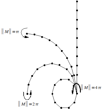
Figure 13.1-a: Beam subjected to an end moment

13.2. Recessed swivel arch loaded at the top

Figure [fig 13.2-a] shows the deformations of an arc with 215° opening, embedded on the right, rotated on the left and subjected to an increasing force concentrated at the top. The solution to this problem is given in [bib11] for an initial radius of 100 and the following beam characteristics:

\(\mathrm{EA}=\mathrm{GA}=5\times {10}^{7}\) and \(\mathrm{EI}={10}^{6}\)

The arc is modelled by 40 first-order elements. The force was increased to 890 by eight increments of 100, one increment of 50, and four increments of 10. Beyond that appears the boom, that is to say that the displacement continues to increase under a force that decreases sharply. The algorithm described here does not make it possible to take such a phenomenon into account, and diverges for a force of 900. Da Deppo, in [bib11], places the critical force at 897.

We have the following table of comparative results:

	Force	Vertical movement of the application point	Horizontal movement of the application point
Our calculations	890	—110.5	—60.2
Da Deppo	897	—113.7	—61.2

Figure 13.2-a: Embedded-swivel arch loaded at the top (Da Deppo)

13.3. Circular arc of 45° embedded and subjected at the end to a force perpendicular to its plane

The problem is three dimensional. It was proposed in [bib12]. Figure [fig 13.3-a] shows three successive configurations of the beam of initial radius 100, of square cross section and of characteristics:

\(\text{EA}={\text{10}}^{7},{\text{GA}}_{1}={\text{GA}}_{2}=5\times {\text{10}}^{6}\text{,}{\text{GI}}_{1}={\text{EI}}_{2}={\text{EI}}_{3}=8\text{.}\text{333}\times {\text{10}}^{5}\text{.}\)

Figure 13.3-a: Three configurations of the beam (taken from [bib12])

We modelled the beam by 8 first-order elements. The force increases in increments of 20. We have the following comparative results, for the coordinates of the point of application of the force, in the configurations in figure [fig 13.3-a].

FORCE		\(X\)		\(Y\)	\(Z\)
300	Our calculations	22.3	22.3	58.9	40.1
	BATHE - BOLOURCHI	22.5	59.2	39.5
600	Our calculations	15.7	15.7	47.3	53.4
	BATHE - BOLOURCHI	15.9	15.9	47.2	53.4

13.4. Movement of a gallows

This is a dynamic three-dimensional problem addressed in [bib3].

A gallows consists of a pole and a crosspiece of length 10 [fig 13.4-a] (a). The foot of the post is embedded and a non-tracking force is applied to the joint, perpendicular to the plane of the stem at rest [fig 13.4-a] (b).

Figure 13.4-a: Crane subjected to a dynamic force perpendicular to its plane

The characteristics of the items provided by [bib3] are as follows:

\(\begin{array}{}\mathrm{EA}=G{A}_{1}=G{A}_{2}={10}^{6}\\ G{I}_{1}=E{I}_{2}=E{I}_{3}={10}^{3}\\ \rho A=1\\ \rho {I}_{2}=\rho {I}_{3}=10;\rho {I}_{1}=20\end{array}\)

We note that this data does not make it possible to identify a material and a section of a beam, because we have at the same time:

\(\frac{{\mathrm{EI}}_{2}}{\rho {I}_{2}}={10}^{2}=\frac{E}{\rho }\text{et}\frac{EA}{\rho A}={10}^{6}=\frac{E}{\rho }\)

We can therefore only deal with this problem by programmatically imposing a characteristic: we have chosen to impose the product \(\mathrm{EA}\).

The column and the crosspiece are each modelled by 4 first-order elements and the duration of the analysis includes 120 equal steps of 0.25.

FIGS. [fig 13.4-b] and [fig 13.4-c] show the evolution of the following component \(x\) of the movement respectively for the connector and for the end of the crosspiece. In cartridge, the corresponding curves given in [bib3] were reproduced for two models.

Figure 13.4-b: Stem of SIMO - Movement of the connection Perpendicular to the initial plane.

Figure 13.4-c: SIMO stem - End displacement Perpendicular to the initial plane.

13.5. Rotation of a robot arm

A robot arm \(\mathrm{OA}\) is set in motion in the \({e}_{1}{e}_{2}\) plane by a rotation \(\Psi (t)\) imposed on its axis 0 [fig 13.5-a]. We want to calculate the displacement of the end \(A\) in a system of axes \({e}_{1}^{’}{e}_{2}^{’}\) driven in the rotation \(\Psi (t)\).

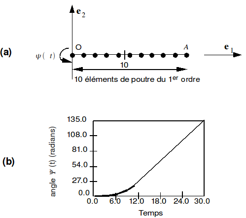
Figure 13.5-a: Robot arm subjected to imposed rotation.

Material characteristics:

\(\begin{array}{}\mathrm{EA}=2.8{10}^{7}\\ {\mathrm{GA}}_{2}={10}^{7}\\ \mathrm{EI}=1.4{10}^{4}\\ A\rho =1.2\\ I\rho =6{10}^{\text{-4}}\end{array}\)

The time step changes from 0.05 at the start of the analysis to 0.001 at the end.

Figures [fig 13.5-b] and [fig 13.5-c] show the evolution of the displacement along \({e}_{1}\text{'}\) and in the perpendicular direction. The corresponding curve of [bib3] has been reproduced in cartridge form. When the speed of rotation becomes constant, the arm undergoes permanent elongation due to centrifugal force and is subjected to a low-amplitude flexural oscillation.

Figure 13.5-b: Next Movement \({e}_{1}\text{'}\)

Figure 13.5-c: Next Movement \({e}_{2}\text{'}\)