15. Description of document versions#
Version Aster |
Author (s) Organization (s) |
Description of changes |
3 |
Mr. Aufaure EDF -R&D/ MMN |
Initial text |
: Some definitions and results concerning third-order antisymmetric matrices To any vector \(u\) of order 3 and of components \({u}_{x},{u}_{y},{u}_{z}\) we can associate the following antisymmetric matrix \(\stackrel{ˆ}{u}\) of order 3:
\(\stackrel{ˆ}{u}=\left[\begin{array}{ccc}0& -{u}_{z}& {u}_{y}\\ {u}_{z}& 0& -{u}_{x}\\ -{u}_{y}& {u}_{x}& 0\end{array}\right]\) eq A1-1
Conversely, any third-order antisymmetric matrix can be written in the form [A1-1] and a \(u\) vector can therefore be associated with it. This vector is called the axial vector of the matrix.
It is easy to see that:
\(\stackrel{ˆ}{u}u=0\) eq A1-2
in other words, the axial vector is the eigenvector of the associated antisymmetric for the eigenvalue 0.
Regardless of vector \(v\):
\(\stackrel{ˆ}{u}v=u\wedge v\) eq A1-3
\(\stackrel{ˆ}{u}\stackrel{ˆ}{v}=v{u}^{T}-(u\text{.}v)1\text{.}\) eq A1-4
If \(u\) is unitary:
\({\stackrel{ˆ}{u}}^{2}={\mathrm{uu}}^{T}\) (symmetric matrix)
\({\stackrel{ˆ}{u}}^{3}=-\stackrel{ˆ}{u}\) (antisymmetric matrix)
From where:
\({\stackrel{ˆ}{u}}^{\mathrm{2p}}={(-1)}^{p-1}{\stackrel{ˆ}{u}}^{2}\) (symmetric matrix) eq A1-5
\({\stackrel{ˆ}{u}}^{\mathrm{2p}-1}={(-1)}^{p-1}\stackrel{ˆ}{u}\) (antisymmetric matrix) eq A1-6
: Treatment of damping forces These steps are not currently taken into account in the*Code_Aster*.
A2.1 Assumptions and elements of reduction in the center of the section
It is assumed that the volume element \(\mathrm{dv}\) adjacent to a point \(M\) inside the beam is subject to a damping force consisting of two parts:
for the translational movement of the x-axis section \(s\) to which \(M\) belongs:
\(d{\overline{f}}_{1}=-{\xi }_{1}{\dot{x}}_{o}(s,t)\text{dv};\)
for the angular speed rotation movement around the center \({P}^{\text{'}}\) of the section:
\(d{\overline{f}}_{2}=-{\xi }_{2}\omega (s,t)\wedge \overrightarrow{P\text{'}M}\text{dv}\text{.}\)
Integrated into the volume of the \(\mathrm{ds}\) length beam, these forces allow for elements of reduction in \({P}^{\text{'}}\):
strength:
\(d\overline{f}=-{\xi }_{1}A{\dot{x}}_{o}(s,t)\text{ds};\)
the moment:
\(d\stackrel{ˉ}{m}=-{\xi }_{2}\mathrm{ds}{\int }_{\mathrm{section}}\overrightarrow{P\text{'}M}\wedge \left[\omega (s,t)\wedge \overrightarrow{P\text{'}M}\right]d\sigma =\frac{-{\xi }_{2}}{\rho }{I}_{\rho }\omega (s,t)\mathrm{ds}\)
A2.2 Elementary damping forces
The virtual work of the damping forces is:
\({W}_{\mathrm{amor}}=-{\int }_{{S}_{1}}^{{S}_{2}}\left\{\begin{array}{c}{\xi }_{1}A\dot{{x}_{0}}\\ \frac{{\xi }_{2}}{\rho }{I}_{\rho }\omega \end{array}\right\}\left\{\begin{array}{c}\delta {x}_{0}\\ \delta \Psi \end{array}\right\}\text{ds}\)
If depreciation is taken into account, \({W}_{\text{amor}}\) should be subtracted from the second member of the equation [éq 9-1].
It follows from this, as in [§10.3] for inertial forces, that the contribution of element \(e\) to the damping force at node \(i\) is:
\({F}_{\text{amor}i}^{e}=-{\int }_{e}\left\{\begin{array}{c}{N}_{i}{\xi }_{1}A\dot{{x}_{0}}\\ {N}_{i}\frac{{\xi }_{2}}{\rho }{I}_{\rho }\omega \end{array}\right\}\text{ds}\)
If damping is taken into account, these forces must be added to the second member of equation [éq10.6‑1].
A2.3 Depreciation matries
Based on the relationships [éq A4-3] and [éq A4-7] giving the Fréchet differentials of \({\dot{x}}_{o}\) and \(\omega\) in the \(\Delta \phi\) direction, and considering that ([éq A4-5] and [éq A4-6]):
\((D{I}_{\rho }\mathrm{.}\Delta \Psi )\omega =\left[-{({I}_{\rho }\omega )}^{\text{^}}+{I}_{\rho }\stackrel{ˆ}{\omega }\right]\Delta \Psi\)
\(D{W}_{\mathrm{amor}}\mathrm{.}\Delta \Phi =-{\int }_{{S}_{1}}^{{S}_{2}}\delta \Phi \mathrm{.}\left[\begin{array}{cc}{\xi }_{1}A1& 0\\ 0& \frac{{\xi }_{2}}{\rho }{I}_{\rho }\end{array}\right]\Delta \dot{\Phi }\mathrm{ds}-{\int }_{{S}_{1}}^{{S}_{2}}\delta \Phi \mathrm{.}\left[\begin{array}{cc}0& 0\\ 0& \frac{-{\xi }_{2}}{\rho }{({I}_{\rho }\omega )}^{\text{^}}\end{array}\right]\Delta \Phi \mathrm{ds}\)
From this we deduce the damping matrices for element \(e\):
to the nearest sign, relationship between the increase in speed at node \(j\) and the increase in damping force at node \(i\):
\({C}_{\mathrm{amor}ij}^{e}={\int }_{e}{N}_{i}{N}_{j}\left[\begin{array}{cc}{\xi }_{1}A1& 0\\ 0& \frac{{\xi }_{2}}{\rho }{I}_{\rho }\end{array}\right]\mathrm{ds}\)
to the nearest sign, relationship between the increase in displacement at node \(j\) and the increase in damping force at node \(i\):
\({S}_{\mathrm{amor}ij}^{e}={\int }_{e}{N}_{i}{N}_{j}\left[\begin{array}{cc}0& 0\\ 0& \frac{-{\xi }_{2}}{\rho }{({I}_{\rho }\omega )}^{\text{^}}\end{array}\right]\mathrm{ds}\)
In the bracket on the first member of equation [éq 10.6.1], add:
the \(\frac{\gamma }{\beta \Delta t}{C}_{\text{amor}};\) matrix
the \({S}_{\text{amor}}\text{.}\) matrix
Matrix \({C}_{\text{amor}}^{e}\text{.}\) is symmetric, but matrix \({S}_{\text{amor}}^{e}\text{.}\) is antisymmetric.
: Newmark algorithm in large rotations A3.1 Classical Newmark schema in translation
The state of the center line (displacement, speed and acceleration) is assumed to be known at time \(i-1\) The Newmark algorithm [bib10] and [bib13], is based on the following developments of displacement and speed, at iteration \(n+1\) of time \(i\):
\({x}_{o,i}^{n+1}={x}_{o,i-1}+\Delta t{\dot{x}}_{o,i-1}+\frac{\Delta {t}^{2}}{2}\left[(1-2\beta ){\ddot{x}}_{o,i-1}+2\beta {\ddot{x}}_{o,i}^{n+1}\right]\) eq A3.1-1
\({\dot{x}}_{o,i}^{n+1}={\dot{x}}_{o,i-1}+\Delta t\left[(1-\gamma ){\ddot{x}}_{o,i-1}+\gamma {\ddot{x}}_{o,i}^{n+1}\right]\) eq A3.1-2
\(\beta ` and :math:\)gamma` are the Newmark parameters which, in the case of the « trapezium rule », are equal to \(\frac{1}{4}\) and \(\frac{1}{2}\): the brackets in the equations [éq A3.1-1] and [éq A3.1-2] are then the arithmetic means of \({\ddot{x}}_{o,i-1}\) and \({\ddot{x}}_{o,i}^{n+1}\)
Rewriting each of these relationships in iteration \(n\) from moment \(i\) and removing member from member from previous relationships, he comes:
\({\ddot{x}}_{o,i}^{n+1}={\ddot{x}}_{o,i}^{n}+\frac{1}{\beta \Delta {t}^{2}}({x}_{o,i}^{n+1}-{x}_{o,i}^{n})\) and \({\dot{x}}_{o,i}^{n+1}={\dot{x}}_{o,i}^{n}+\frac{\gamma }{\beta \Delta t}({x}_{o,i}^{n+1}-{x}_{o,i}^{n})\)
If one asks:
\({x}_{o,i}^{n+1}={x}_{o,i}^{n}+\Delta {x}_{o,i}^{n+1},\) eq A3.1-3
So we have:
\({\ddot{x}}_{o,i}^{n+1}={\ddot{x}}_{o,i}^{n}+\frac{1}{\beta \Delta {t}^{2}}\Delta {x}_{o,i}^{n+1}\) and \({\dot{x}}_{o,i}^{n+1}={\dot{x}}_{o,i}^{n}+\frac{\gamma }{\beta \Delta t}\Delta {x}_{o,i}^{n+1}\) eq A3.1-4
A3.2 Newmark diagram adapted to large rotations
To unify the calculations, we would like to be able to write, in rotation, the following analogous relationships:
\({\omega }_{i}^{n+1}={\omega }_{i}^{n}+\frac{\gamma }{\beta \Delta t}({\Psi }_{i-\mathrm{1,}i}^{n+1}-{\Psi }_{i-\mathrm{1,}i}^{n})\) and \({\dot{\omega }}_{i}^{n+1}={\dot{\omega }}_{i}^{n}+\frac{1}{\beta \Delta {t}^{2}}({\Psi }_{i-\mathrm{1,}i}^{n+1}-{\Psi }_{i-\mathrm{1,}i}^{n})\)
where \({\Psi }_{i-\mathrm{1,}i}^{n}\) and \({\Psi }_{i-\mathrm{1,}i}^{n+1}\) are respectively the rotation increment vectors of the section in question, between the instant \(i-1\) and the iterations \(n\) and \(n+1\) of the instant \(i\) [A6].
But these relationships are not exact because you cannot combine an angular speed (or acceleration) at iteration (\(n+1\)) from time \(i\) with the quantity equivalent to iteration \(n\) and rotation vectors counted from the configuration at time \(i-1\) [A7]. It is only possible to combine all the quantities after having rotated (we say « transported ») all the quantities in the same configuration. To simplify the reference configuration, the reference configuration is chosen.
So let’s say:
\({\Omega }_{i}^{n+1}={R}_{i}^{n+\mathrm{1,}T}{\omega }_{i}^{n+1}\text{}{\Omega }_{i}^{n}={R}_{i}^{n,T}{\omega }_{i}^{n}\) eq A3.2-1
\({A}_{i}^{n+1}={R}_{i}^{n+\mathrm{1,}T}{\dot{\omega }}_{i}^{n+1}\text{}{A}_{i}^{n}={R}_{i}^{n,T}{\dot{\omega }}_{i}^{n}\) eq A3.2-2
\({\Psi }_{i-\mathrm{1,}i}^{n+1}={R}_{i-1}^{T}{\Psi }_{i-\mathrm{1,}i}^{n+1}\text{}{\Psi }_{i-\mathrm{1,}i}^{n}={R}_{i-1}^{T}{\Psi }_{i-\mathrm{1,}i}^{n}\)
The Newmark algorithm in rotation results in the following relationships:
for the rotation operator, [éq A6-1]:
\({R}_{i}^{n+1}=\text{exp}(\stackrel{ˆ}{{\Delta \Psi }_{i}^{n+1}}){R}_{i}^{n};\)
for the rotation-vector increment since instant \(i-1\), [éq A6-2]:
\(\text{exp}({\stackrel{ˆ}{\Psi }}_{i-\mathrm{1,}i}^{n+1})=\text{exp}(\stackrel{ˆ}{{\Delta \Psi }_{i}^{n+1}})\text{exp}({\stackrel{ˆ}{\Psi }}_{i-\mathrm{1,}i}^{n});\)
for angular speed:
\({\Omega }_{i}^{n+1}={\Omega }_{i}^{n}+\frac{\gamma }{\beta \Delta t}({\Psi }_{i-\mathrm{1,}i}^{n+1}-{\Psi }_{i-\mathrm{1,}i}^{n});\)
for angular acceleration:
\({A}_{i}^{n+1}={A}_{i}^{n}+\frac{1}{\beta \Delta {t}^{2}}({\Psi }_{i-\mathrm{1,}i}^{n+1}-{\Psi }_{i-\mathrm{1,}i}^{n})\text{.}\)
The two previous relationships give, by reverse transport on configuration \((\begin{array}{c}n+1\\ i\end{array})\) and taking into account the relationships [éq A3.2-1] and [éq A3.2-2]:
\({\omega }_{i}^{n+1}={R}_{i}^{n+1}{R}_{i}^{n,T}{\omega }_{i}^{n}+\frac{\gamma }{\beta \Delta t}{R}_{i}^{n+1}{R}_{i-1}^{T}({\Psi }_{i-\mathrm{1,}i}^{n+1}-{\Psi }_{i-\mathrm{1,}i}^{n})\) eq A3.2-3
\({\dot{\omega }}_{i}^{n+1}={R}_{i}^{n+1}{R}_{i}^{n,T}{\dot{\omega }}_{i}^{n}+\frac{1}{\beta \Delta {t}^{2}}{R}_{i}^{n+1}{R}_{i-1}^{T}({\Psi }_{i-\mathrm{1,}i}^{n+1}-{\Psi }_{i-\mathrm{1,}i}^{n})\text{.}\) eq A3.2-4
: Calculation of Fréchet differentials We will then have to use the following identity, called Lie hook, whose demonstration is immediate. If \(\stackrel{ˆ}{A}\) and \(\stackrel{ˆ}{B}\) are two antisymmetric matrices of the 3rd order, with axial vectors \(A\) and \(B\), then we have, for any vector \(v\):
\((\stackrel{ˆ}{A}\stackrel{ˆ}{B}-\stackrel{ˆ}{B}\stackrel{ˆ}{A})v=(A\wedge B)\wedge v\) eq A4-1
In other words: is the axial vector of the antisymmetric matrix \(\stackrel{ˆ}{A}\stackrel{ˆ}{B}-\stackrel{ˆ}{B}\stackrel{ˆ}{A}\).
We call the Fréchet differential of the function \(f\) in the \(\Delta x\) direction, the quantity:
\(Df(x)\text{.}\Delta x=\text{grad}f\text{.}\Delta x=\underset{\varepsilon \to 0}{\text{lim}}\frac{d}{d\varepsilon }f(x+\varepsilon \Delta x)\text{.}\)
This is the main part of the increase in \(f\) corresponding to the increase \(\Delta x\) in the variable \(x\).
Here is the catalog of the Fréchet differentials used in this note.
\(D{x}_{o}\text{'}\text{.}\Delta {x}_{o}=\underset{\varepsilon \to 0}{\text{lim}}\frac{d}{d\varepsilon }({x}_{o}+\varepsilon \Delta {x}_{o})\text{'}=(\Delta {x}_{o})\text{'}=\Delta {x}_{o}\text{'}\) eq A4-2
\(D{\dot{x}}_{o}\text{.}\Delta {x}_{o}=\Delta {\dot{x}}_{o}\) eq A4-3
\(D{\ddot{x}}_{o}\text{.}\Delta {x}_{o}=\Delta {\ddot{x}}_{o}\) eq A4-4
\(DR\text{.}\Delta \Psi =\underset{\varepsilon \to 0}{\text{lim}}\frac{d}{d\varepsilon }\left[\text{exp}(\varepsilon \stackrel{ˆ}{\Delta \Psi })R\right]=\stackrel{ˆ}{\Delta \Psi }R\) eq A4-5
\(D{R}^{T}\text{.}\Delta \Psi =\underset{\varepsilon \to 0}{\text{lim}}\frac{d}{d\varepsilon }\left[{R}^{T}\text{exp}(-\varepsilon \stackrel{ˆ}{\Delta \Psi })\right]=-{R}^{T}\stackrel{ˆ}{\Delta \Psi }\) eq A4-6
because, according to equation [éq 4.2-6]:
\({\left[\text{exp}(\varepsilon \stackrel{ˆ}{\Delta \Psi })\right]}^{T}=\text{exp}(-\varepsilon \stackrel{ˆ}{\Delta \Psi })\text{.}\)
\(\stackrel{ˆ}{\omega }=\dot{R}{R}^{T}\text{.}\)
Gold:
\(D\dot{R}\text{.}\Delta \Psi =\underset{\varepsilon \to 0}{\text{lim}}\frac{d}{d\varepsilon }{\left[\text{exp}(\varepsilon \stackrel{ˆ}{\Delta \Psi })R\right]}^{·}=\stackrel{ˆ}{\Delta \dot{\Psi }}R+\stackrel{ˆ}{\Delta \Psi }\dot{R}\text{.}\)
So, according to [éq A4-6]:
\(D\stackrel{ˆ}{\omega }\text{.}\Delta \Psi =(D\dot{R}\text{.}\Delta \Psi ){R}^{T}+\dot{R}(D{R}^{T}\text{.}\Delta \Psi )=\stackrel{ˆ}{\Delta \dot{\Psi }}+\stackrel{ˆ}{\Delta \Psi }\stackrel{ˆ}{\omega }-\stackrel{ˆ}{\omega }\stackrel{ˆ}{\Delta \Psi }\text{.}\)
Or, using the Lie hook [éq A4-1]:
\(D\omega \text{.}\Delta \Psi =\Delta \dot{\Psi }-\omega \wedge \Psi\) eq A4-7
: Complements on the calculation of stiffness matrices This appendix develops the calculations for [§9.1].
A5.1 Geometric stiffness matrix
\(\begin{array}{}\left[D\left\{B\delta \phi \right\}\text{.}\Delta \phi \right]\text{.}\Pi \left\{\begin{array}{c}F\\ M\end{array}\right\}+\left\{B\delta \phi \right\}\text{.}\left[D\Pi \text{.}\Delta \phi \right]\left\{\begin{array}{c}F\\ M\end{array}\right\}=\\ (\Delta {x}_{o}\text{'}\wedge \delta \Psi )\text{.}f+(\delta {x}_{o}\text{'}+{x}_{o}\text{'}\wedge \delta \Psi )\text{.}\stackrel{ˆ}{\Delta \Psi }f+\delta \Psi \text{'}\text{.}\stackrel{ˆ}{\Delta \Psi }m\text{.}\end{array}\)
By rearranging terms and using vector identity:
\(a\text{.}(b\wedge c)=c\text{.}(a\wedge b),\)
The second previous member is written as:
\(-\delta {x}_{o}\text{'}\text{.}f\wedge \Delta \Psi -\delta \Psi \text{'}\text{.}m\wedge \Delta \Psi +\delta \Psi \text{.}f\wedge \Delta {x}_{o}\text{'}+\delta \Psi \text{.}({\stackrel{ˆ}{x}}_{o}\text{'}\stackrel{ˆ}{f})\Delta \Psi =Y\delta \phi \text{.}EY\Delta \phi \text{.}\)
A5.2 Material and complementary stiffness matries
As shown in [§9.1]:
\(D\left\{\begin{array}{c}F\\ M\end{array}\right\}\text{.}\Delta \phi =C{\Pi }^{T}B\Delta \phi -C{\Pi }^{T}(\begin{array}{cc}\stackrel{ˆ}{\Delta \Psi }& 0\\ 0& \stackrel{ˆ}{\Delta \Psi }\end{array})\left\{\begin{array}{c}\varepsilon \\ \chi \end{array}\right\}\text{.}\)
Gold:
\(\left\{\begin{array}{c}\varepsilon \\ \chi \end{array}\right\}=\Pi {C}^{-1}{\Pi }^{T}\left\{\begin{array}{c}f\\ m\end{array}\right\}\text{.}\)
Therefore:
\(\left\{B\delta \phi \right\}\text{.}\Pi (D\left\{\begin{array}{c}F\\ M\end{array}\right\}\text{.}\Delta \phi )=\left\{B\delta \phi \right\}\text{.}\Pi C{\Pi }^{T}B\Delta \phi\) eq A5.2-1
\(-\left\{B\delta \phi \right\}\text{.}\Pi C{\Pi }^{T}(\begin{array}{cc}\stackrel{ˆ}{\Delta \Psi }& 0\\ 0& \stackrel{ˆ}{\Delta \Psi }\end{array})\Pi {C}^{\pm 1}{\Pi }^{T}\left\{\begin{array}{c}f\\ m\end{array}\right\}\text{.}\)
The term:
\(\left\{B\delta \phi \right\}\text{.}\Pi C{\Pi }^{T}B\Delta \phi\)
immediately leads to the material stiffness matrix.
On the other hand:
\((\begin{array}{cc}\stackrel{ˆ}{\Delta \Psi }& 0\\ 0& \stackrel{ˆ}{\Delta \Psi }\end{array})\Pi {C}^{-1}{\Pi }^{T}\left\{\begin{array}{c}f\\ m\end{array}\right\}=-\left\{\begin{array}{c}{({R}_{\text{tot}}{C}_{1}^{-1}{R}_{\text{tot}}^{T}f)}^{\wedge }\Delta \Psi \\ {({R}_{\text{tot}}{C}_{2}^{-1}{R}_{\text{tot}}^{T}m)}^{\wedge }\Delta \Psi \end{array}\right\}\text{.}\)
So the second term in equation [éq A5.2-1] is written as:
\(B\delta \phi \text{.}\left[\begin{array}{cc}0& {R}_{\text{tot}}{C}_{1}{R}_{\text{tot}}^{T}{({R}_{\text{tot}}{C}_{1}^{\pm 1}{R}_{\text{tot}}^{T}f)}^{\wedge }\\ 0& {R}_{\text{tot}}{C}_{2}{R}_{\text{tot}}^{T}{({R}_{\text{tot}}{C}_{2}^{\pm 1}{R}_{\text{tot}}^{T}m)}^{\wedge }\end{array}\right]\Delta \phi \text{.}\)
By designating the matrix in square brackets in the preceding expression by \(Z\), \({B}^{t}Z\) is the complementary stiffness matrix.
: Principle of iterative rotation calculation This appendix visualizes the exponentiation operation, defines the rotation increment vectors that occur in appendix 3, and gives the relationship between them.
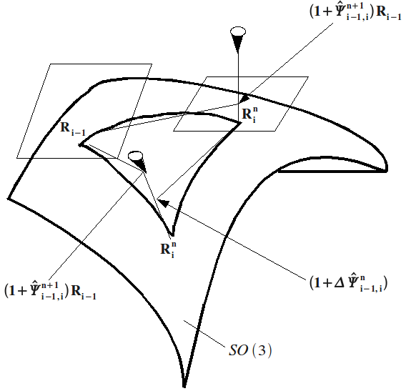
Figure A6-a: Representation of the operators involved in the rotation of sections. : symbol of the exponential projection
The curved surface in figure [fig. A6-a] represents the set \(\mathrm{SO}(3)\) of rotation operators \(R\). The spaces tangent to \(\mathrm{SO}(3)\) were shown in \({R}_{i-1}\), rotation calculated at time \(i-1\), and in, \(n\) \({R}_{i}^{n}\) -th iteration in calculating the rotation at time \(i\).
Let \({\Psi }_{i-1}\) be the rotation vector corresponding to. \({R}_{i-1}\) There is a \({\Psi }_{i-\mathrm{1,}i}^{n}\) rotation increment vector such as:
\({R}_{i}^{n}=\text{exp}({\stackrel{ˆ}{\Psi }}_{i-\mathrm{1,}i}^{n}){R}_{i-1}\text{.}\)
If the balance equation of the beam is not satisfied, at time \(i\), by \({R}_{i}^{n}\), we look for a correction \(\Delta {\Psi }_{i}^{n+1}\text{de}{\Psi }_{i-\mathrm{1,}i}^{n}\text{.}\Delta {\Psi }_{i}^{n+1}\) is obtained by linearization, by replacing in the equilibrium equation, according to the equivalence [éq 4.2-5]:
\(\text{exp}\stackrel{ˆ}{{\Delta \Psi }_{i}^{n+1}}{R}_{i}^{n}\text{par}(1+\stackrel{ˆ}{{\Delta \Psi }_{i}^{n+1}}){R}_{i}^{n}\text{.}\)
The second of the previous expressions is not a rotation operator, but is in space tangent to \(\mathrm{SO}(3)\) in \({R}_{i}^{n}\) [fig A6-a]. Having calculated \(\Delta {\Psi }_{i}^{n+1},{R}_{i}^{n+1}\) can be deduced by projecting by exp to \(\mathrm{SO}(3)\):
\({R}_{i}^{n+1}=\text{exp}(\stackrel{ˆ}{{\Delta \Psi }_{i}^{n+1}}){R}_{i}^{n}\text{.}\) eq A6-1
The rotation angle increment \({\Psi }_{i-\mathrm{1,}i}^{n+1}\) to go from \({R}_{i-1}\) to \({R}_{i}^{n+1}\) is such that:
\({R}_{i}^{n+1}=\text{exp}({\stackrel{ˆ}{\Psi }}_{i-\mathrm{1,}i}^{n+1}){R}_{i-1}\text{.}\)
Since the rotation vectors are not additive, we don’t:
\({\Psi }_{i-\mathrm{1,}i}^{n+1}=\Delta {\Psi }_{i}^{n+1}+{\Psi }_{i-\mathrm{1,}i}^{n},\)
but we have:
\(\text{exp}({\stackrel{ˆ}{\Psi }}_{i-\mathrm{1,}i}^{n+1})=\text{exp}(\stackrel{ˆ}{{\Delta \Psi }_{i}^{n+1}})\text{exp}({\stackrel{ˆ}{\Psi }}_{i-\mathrm{1,}i}^{n})\) eq A6-2
In [§10.7.2], we solve the previous equation with respect to \({\Psi }_{i-\mathrm{1,}i}^{n+1}\) using the properties of quaternions.
Rotation angle increments \({\Psi }_{i-\mathrm{1,}i}^{n}\text{et}{\Psi }_{i-\mathrm{1,}i}^{n+1}\) are used to calculate speed and acceleration corrections from \((\begin{array}{c}n\\ i\end{array})\) to \((\begin{array}{c}n+1\\ i\end{array})\).
: The need for transport in a reference space for vector operations relating to rotational movement The kinematic quantities, velocities and accelerations, in a given configuration, are found in the vector space tangent to \(\mathrm{SO}(3)\) at the point defined by the rotation of the configuration with respect to the reference position. Quantities relating to two distinct configurations can only be combined after having transported them in the same vector space taken as a reference. The following example will illustrate this need.
Let’s look at the angular speed of a gyroscope at three times \({t}_{1},{t}_{2}\) and \({t}_{3}\) [fig A7-a]. Assume that we go from configuration 1 to configuration 2 by rotating the angle \(-\pi\) around \({e}_{1}\), and from the configuration 1 to the configuration 3 by rotating the angle \(-\pi /2\) around the same axis. In 1, the angular speed is carried by the gyro axis and has \((\mathrm{0,}\mathrm{0,}\omega )\) components in the general \({e}_{1}\text{}{e}_{2}\text{}{e}_{3}\) axes. In 2, the angular speed is also carried by the axis and has \((\mathrm{0,}\mathrm{0,}–3\omega )\) as general components. We want to determine the general components of the speed in 3, knowing that this speed is the average of the speeds in 1 and 2.
That the angular speed in 3 is the average of the angular velocities in 1 and 2 does not mean that it is the average in the general axes, but in the axes related to the gyro. In the example, since the gyro rotates around its axis, in 1 with speed \(\omega\), in 2 with speed 3 \(\omega\), then in 3 it rotates around this axis with speed \(2\omega\). So in 3, the general components of angular velocity are \((\mathrm{0,}2\omega ,0)\).
Taking into account [§5], the previous result is obtained by « transporting » the angular velocity vector from configuration 2 to configuration 1, taken as a reference, i.e. by rotating this vector from the angle \(\pi\) around \({e}_{1}\). Its general components are then \((\mathrm{0,}\mathrm{0,}3\omega )\). We average this vector and the angular velocity vector at 1, to obtain the component vector \((\mathrm{0,}\mathrm{0,}2\omega )\). We finally « transport » this last vector to configuration 3 by making it rotate from \(-\pi /2\) around \({e}_{1}\), and we end up with the angular velocity vector with general components \((\mathrm{0, 2}\omega ,0)\).
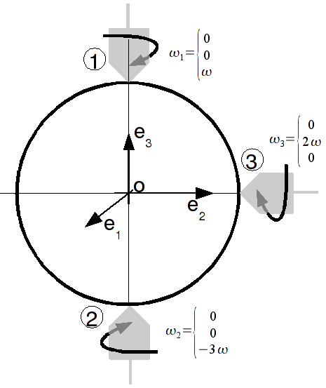
Figure A7-a: Evolution of the angular speed of a gyroscope.
: Use of quaternions in modeling large rotations [bib14] [bib15] A8.1 Definitions
A quaternion, noted \((q)\) or \(({x}_{o},x)\), is defined by the set of a scalar \({x}_{o}\) and a three-dimensional vector \(x({x}_{1}\text{}{x}_{2}\text{}{x}_{3})\):
\(({x}_{o},x)={x}_{o}+{x}_{1}\iota +{x}_{2}\kappa +{x}_{3}\lambda ,\),
\(\iota ,\kappa\) and \(\lambda\) being three numbers satisfying relationships:
\(\begin{array}{}{\iota }^{2}={\kappa }^{2}={\lambda }^{2}=-1;\\ \iota \kappa =-\kappa \iota =\lambda ;\kappa \lambda =-\lambda \kappa =\iota ;\lambda \iota =-\iota \lambda =\kappa \text{.}\end{array}\)
Conjugated quaternion
The conjugate, noted \({}^{\ast }\), of a quaternion is obtained by changing the sign of the vector part:
\({({x}_{o},x)}^{\ast }=({x}_{o},-x)\text{.}\)
Purely vector quaternion
A quaternion is said to be purely vector when its scalar part is zero and it is therefore of the form: \((\text{0,}x)\). A quaternion \((v)\) is purely vectorial if and only if:
\((v)+{(v)}^{\ast }=(0)\text{.}\)
A8.2 Quaternion Algebra Elements
Multiplication
Applying the definition, we immediately show that the multiplication, noted \(°\), of two quaternions is:
\(({x}_{o},x)°({y}_{o},y)=({x}_{o}{y}_{o}-x\text{.}y,{x}_{o}y+{y}_{o}x+x\wedge y)\text{.}\)
We check that this multiplication is:
associative:
\(\left[({x}_{o},x)+({y}_{o},y)\right]°({z}_{o},z)=({x}_{o},x)°({z}_{o},z)+({y}_{o},y)°({z}_{o},z);\)
not commutative because:
\(({x}_{o},x)°({y}_{o},y)-({y}_{o},y)°({x}_{o},x)=(\mathrm{0,2}x\wedge y)\text{.}\)
Standard of a quaternion, noted \(\parallel \text{.}\parallel\):
\({\parallel ({x}_{o},x)\parallel }^{2}=({x}_{o},x)°{({x}_{o},x)}^{\ast }={x}_{0}^{2}+{x}_{1}^{2}+{x}_{2}^{2}+{x}_{3}^{2}\text{.}\)
A quaternion is unitary if its norm is equal to unity. It is verified that:
\({\left[({q}_{1})°({q}_{2})\right]}^{\ast }={({q}_{2})}^{\ast }°{({q}_{1})}^{\ast }\text{.}\)
A8.3 Representation of a rotation by a quaternion
If \(({v}_{1})\) is a purely vector quaternion and \((u)\) is a unit quaternion, then quaternion \(({v}_{2})\) such that:
\(({v}_{2})=(u)°({v}_{1})°{(u)}^{\ast }\) eq A8.3-1
is purely vectorial and has the same standard as \(({v}_{1})\). In fact:
\(\begin{array}{}({v}_{2})+{({v}_{2})}^{\ast }=(u)°({v}_{1})°{(u)}^{\ast }+(u)°({v}_{1}^{\ast })°{(u)}^{\ast }\\ \text{}=(u)°\left[({v}_{1})+{({v}_{1})}^{\ast }\right]°{(u)}^{\ast }=(0);\\ ({v}_{2})°{({v}_{2})}^{\ast }=(u)°({v}_{1})°{(u)}^{\ast }°(u)°{({v}_{1})}^{\ast }°{(u)}^{\ast }={\parallel ({v}_{1})\parallel }^{2}\text{.}\end{array}\)
If one asks:
\(({v}_{1})=(\text{0,}x);({v}_{2})=(\text{0,}y)\),
we can see that, through the relationship [éq A8.3-1], the unit quaternion \((u)\) defines an orthogonal transformation of the vector \(x\) on the vector \(y\). This transformation is the rotation whose matrix is defined by [éq A8.5-1].
Reverse rotation is defined by quaternion \({(u)}^{\text{*}}\), because:
\({(u)}^{\ast }°({v}_{2})°(u)={(u)}^{\ast }°(u)°({v}_{1})°{(u)}^{\ast }°(u)=({v}_{1})\text{.}\)
A8.4 Successive rotations
Let the purely vector quaternion \(({v}_{1})\) undergo two successive rotations defined by the unit quaternions \(({u}_{1})\text{et}({u}_{2})\):
\(({v}_{2})=({u}_{1})°({v}_{1})°{({u}_{1})}^{\ast }\)
and:
\(({v}_{3})=({u}_{2})°({v}_{2})°{({u}_{2})}^{\ast }=({u}_{2})°({u}_{1})°({v}_{1})°{\left[({u}_{2})°({u}_{1})\right]}^{\ast }\) eq A8.4-1
We can see on the last member of [éq A8.4-1] that the unit quaternion defining the product of two rotations is equal to the product of the quaternions of these rotations.
A8.5 Matrix expressions
Let \((q)\) be a quaternion:
\((q)(q)=({x}_{o},x)\).
Let’s say:
\(\underline{(q)}=\left\{\begin{array}{c}{x}_{o}\\ x\end{array}\right\},\)
\(\underline{(q)}\) is the vector formed by the four components of the quaternion.
Let’s define two matrices built on \((q)\):
\({A}_{(q)}=\left[\begin{array}{cc}{x}_{o}& -{x}^{T}\\ x& {x}_{o}1+\stackrel{ˆ}{x}\end{array}\right]\text{et}{B}_{(q)}=\left[\begin{array}{cc}{x}_{o}& -{x}^{T}\\ x& {x}_{o}1-\stackrel{ˆ}{x}\end{array}\right]\text{.}\)
It is easy to verify, according to the multiplication rule, that:
\(\underline{({q}_{1})°({q}_{2})}={A}_{({q}_{1})}\underline{({q}_{2})}={B}_{({q}_{2})}\underline{({q}_{1})}\).
Now let’s take the rotation defined by the unit quaternion \((u)=({e}_{o},e)\). If:
\(({v}_{2})=(u)({v}_{1}){(u)}^{\ast }\).
So:
\(\underline{({v}_{2})}={A}_{(u)}{B}_{(u)}^{T}\underline{({v}_{1})}\).
On the other hand:
\({A}_{(u)}{B}_{(u)}^{T}=\left[\begin{array}{cc}1& {0}^{T}\\ 0& R\end{array}\right]\),
with:
\(R={\mathrm{ee}}^{T}+{e}_{o}^{2}1+2{e}_{o}\stackrel{ˆ}{e}+{\stackrel{ˆ}{e}}^{2}\),
or, using the [éq A1-4] relationship:
\(R=(2{e}_{o}^{2}-1)1+2({\mathrm{ee}}^{T}+{e}_{o}\stackrel{ˆ}{e})\) eq A8.5-1
Comparing the previous relationship to equation [éq 4.2-3], we see that the components of the unit quaternion defining a rotation are none other than the Euler parameters of this rotation.
A8.6 Passage from a rotation vector to the associated quaternion and vice-versa
The \(Q\) operator that switches from a \(\Psi\) rotation vector to the associated quaternion is defined by the relationships [éq4.2‑2]:
\({e}_{o}=\text{cos}(\frac{1}{2}\parallel \Psi \parallel )\) eq A8.6-1
\(e=\text{sin}(\frac{1}{2}\parallel \Psi \parallel )\frac{\Psi }{\parallel \Psi \parallel }\) eq A8.6-2
Operator \({Q}^{-1}\) is less simple because the inverse of a trigonomitric function does not have a unique determination.
But we notice on [éq 10.7.2-1] and [éq 10.7.2-2] that \({Q}^{-1}\) is used to calculate the rotation-vector \({\Psi }^{n+1}\) deduced from the rotation-vector \({\Psi }^{n}\) by the correction \(\Delta {\Psi }^{n+1}\). In general:
\(\parallel \Delta {\Psi }^{n+1}\parallel \text{<<}\parallel {\Psi }^{n}\parallel\).
We therefore adopted the following strategy: among all the determinations of the vector \({\Psi }^{n+1}\), we take the one whose module is closest to:
\(\parallel \Delta {\Psi }^{n+1}+{\Psi }^{n}\parallel\).
In the case plan, this strategy is rigorous [§ 4.1], but in the three-dimensional case it is not rigorous because:
\(\Delta {\Psi }^{n+1}+{\Psi }^{n}\ne {\Psi }^{n+1}\).
From [éq A8.6-1], we get:
\(\frac{1}{2}\parallel {\Psi }^{n+1}\parallel =\pm {\text{cos}}^{-1}({e}_{o})+\mathrm{2k}\pi\).
The strategy adopted leads to a single determination of \(\frac{1}{2}\parallel {\Psi }^{n+1}\parallel\).
[éq A8.6-2] Then give:
\({\Psi }^{n+1}=2\frac{\frac{1}{2}\parallel {\Psi }^{n+1}\parallel }{\text{sin}(\frac{1}{2}\parallel {\Psi }^{n+1}\parallel )}e\text{.}\)