\[\newcommand{\vector}[1]{\underline{#1}} \newcommand{\vectorZero}{\vector{0}} \newcommand{\tensTwo}[1]{\boldsymbol{#1}} \newcommand{\tensTwoZero}{\tensTwo{0}} \newcommand{\tensTwoUnit}{\tensTwo{I}} \newcommand{\tensFour}[1]{\mathbb{#1}} \newcommand{\inverse}[1]{{#1}^{-1}} \newcommand{\transpose}[1]{{#1}^{T}} \newcommand{\inverseTranspose}[1]{ {#1}^{-T}} \newcommand{\vectorCmpCO}[2]{#1_{\left(#2\right)}} \newcommand{\vectorCmpCT}[2]{#1^{\left(#2\right)}} \newcommand{\tensTwoCmpCO}[3]{#1_{\left(#2 #3\right)}} \newcommand{\tensTwoCmpCT}[3]{#1^{\left(#2 #3\right)}} \newcommand{\tensTwoInva}[2]{I^{#1}_{#2}} \newcommand{\tensTwoDevia}[1]{\boldsymbol{\tilde{#1}}} \newcommand{\tensFourCmpCO}[5]{#1_{\left(#2 #3 #4 #5\right)}} \newcommand{\tensFourCmpCT}[5]{#1^{\left(#2 #3 #4 #5\right)}} \newcommand{\domain}{\Omega} \newcommand{\domainRefe}{\domain^{0}} \newcommand{\domainCurr}{\domain^{t}} \newcommand{\bound}{\partial\domain} \newcommand{\boundRefe}{\bound^{0}} \newcommand{\boundCurr}{\bound^{t}} \newcommand{\boundN}{\bound_{\textrm{N}}} \newcommand{\boundNRefe}{\boundN^{0}} \newcommand{\boundNCurr}{\boundN^{t}} \newcommand{\boundD}{\bound_{\textrm{D}}} \newcommand{\boundDRefe}{\boundD^{0}} \newcommand{\boundDCurr}{\boundD^{t}} \newcommand{\normal}{\vector{n}} \newcommand{\normalRefe}{\normal^{0}} \newcommand{\normalCurr}{\normal^{t}} \newcommand{\posi}{\vector{x}} \newcommand{\posiRefe}{\posi^{0}} \newcommand{\posiCurr}{\posi^{t}} \newcommand{\disp}{\vector{u}} \newcommand{\dispVirt}{\delta\vector{v}} \newcommand{\funcTransfor}{\vector{\varphi}^{t}} \newcommand{\gradTransfor}{\tensTwo{F}} \newcommand{\jacobTransfor}{J} \newcommand{\posiIncr}{\vector{dx}} \newcommand{\posiIncrRefe}{\posiIncr^{0}} \newcommand{\posiIncrCurr}{\posiIncr^{t}} \newcommand{\strainCmp}{\varepsilon} \newcommand{\strain}{\tensTwo{\strainCmp}} \newcommand{\EGLCmp}{E} \newcommand{\ECGDroiteCmp}{C} \newcommand{\ECGGaucheCmp}{B} \newcommand{\ELOGCmp}{{E}_{ln}} \newcommand{\EGL}{\tensTwo{\EGLCmp}} \newcommand{\ECGDroite}{\tensTwo{\ECGDroiteCmp}} \newcommand{\ECGGauche}{\tensTwo{\ECGGaucheCmp}} \newcommand{\ELOG}{\tensTwo{\ELOGCmp}} \newcommand{\EDilCmp}{C^{\star}} \newcommand{\EDil}{\tensTwo{\EDilCmp}} \newcommand{\divTensTwo}[1]{\vector{\nabla} {\cdot} #1 } \newcommand{\divVector}[1]{\vector{\nabla} {\cdot} #1 } \newcommand{\gradScal}[1]{\vector{\nabla} \times #1 } \newcommand{\gradVector}[1]{\vector{\nabla} \times #1 } \DeclareMathOperator{\rand}{rand} \DeclareMathOperator{\round}{round} \DeclareMathOperator{\trace}{trace} \newcommand{\metric} {\tensTwo{g}} \newcommand{\vectorBaseCV}[1]{\vector{g_{#1}}} \newcommand{\vectorBaseCT}[1]{\vector{g^{#1}}} \newcommand{\metricRefe} {\metric^{t}} \newcommand{\metricCurr} {\metric^{0}} \newcommand{\discVect}[1]{\lbrace #1 \rbrace} \newcommand{\discVectLigne}[1]{\langle #1 \rangle} \newcommand{\discVectZero}{\discVect{0}} \newcommand{\discVectCmp}[2]{\lbrace #1 \rbrace_{(#2)}} \newcommand{\discVectLigneCmp}[2]{\langle #1 \rangle_{(#2)}} \newcommand{\discMatr}[1]{\left[ #1 \right]} \newcommand{\discMatrZero}{\discMatr{0}} \newcommand{\discMatrCmp}[3]{\left[ #1 \right]_{(#2#3)}} \newcommand{\onQuadPoint}[2]{{#1}_{#2}} \newcommand{\onNode}[2]{{#1}^{#2}} \newcommand{\quadOrder}{k_{Q}} \newcommand{\nbQuadPoint}{n_Q} \newcommand{\quadWeight}[1]{\omega_{#1}} \newcommand{\quadPointIndex}{i_{\textrm{pg}}} \newcommand{\nodeIndex}{i_{\textrm{no}}} \newcommand{\pres}{p} \newcommand{\presRefe}{\pres^{0}} \newcommand{\presCurr}{\pres^{t}} \newcommand{\stressCmp}{\sigma} \newcommand{\stress}{\tensTwo{\stressCmp}} \newcommand{\stressPKTwoCmp}{S} \newcommand{\stressPKTwo}{\tensTwo{\stressPKTwoCmp}} \newcommand{\work}[1]{W^{#1}} \newcommand{\enerInterne}{\Psi_i} \newcommand{\yieldStress}{\sigmaCmp_{Y}} \newcommand{\youngModulus}{E} \newcommand{\youngModulusCplx}{E^{\star}} \newcommand{\poissonCoef}{\nu} \newcommand{\poissonCoefCplx}{\nu^{\star}} \newcommand{\shearModulus}{G} \newcommand{\bulkModulus}{K} \newcommand{\modulusTangent}{\tensFour{K}} \newcommand{\anglDila}{\psi} \newcommand{\anglFric}{\varphi} \newcommand{\cohesion}{c} \newcommand{\presCapi}{\pres_{c}} \newcommand{\presEau}{\pres_{w}} \newcommand{\presAir}{\pres_{a}} \newcommand{\shapeFunc}{\Phi} \newcommand{\shapeDFunc}{B} \newcommand{\measLine}{\, \mathrm{d} l} \newcommand{\measDomain}{\, \mathrm{d} \domain} \newcommand{\measBound}{\, \mathrm{d} \Gamma} \newcommand{\normEucl}[1]{\Vert{#1} \Vert } \newcommand{\derivee}[2]{#1_{, #2}} \newcommand{\soundSpeed}{c} \newcommand{\soundSpeedComp}{c_{P}} \newcommand{\soundSpeedCisa}{c_{S}} \newcommand{\posiTang}{\posi_{\tau}} \newcommand{\posiNorm}{{x}_{n}} \newcommand{\dispTang}{\disp_{\tau}} \newcommand{\dispNorm}{{u}_{n}} \newcommand{\basisVector}[1]{\vector{e}_{#1}} \newcommand{\sigmVector}{\vector{t}} \newcommand{\sigmVectorTang}{\sigmVector_{\tau}} \newcommand{\sigmVectorNorm}{t_{n}} \newcommand{\lameLambda}{\lambda} \newcommand{\lameMu}{\mu}\]

1. Hyper-elastic formulation#

1.1. Cinematics#

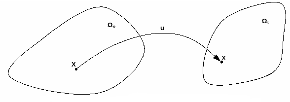
We consider a solid \(\domain\) subject to great deformations. Let \(\gradTransfor\) be the transformation gradient tensor making the initial configuration \({\Omega }_{0}\) go from the initial configuration to the current deformed configuration \(\domainCurr\). We note \(\posiRefe\) the position of a point in \(\domainRefe\) and \(\posiCurr\) the position of this same point after deformation in \(\domainCurr\). \(\disp\) is then the displacement between the two configurations. So we have:

(1.1)#\[ \ PosiCurr =\ PosiRefe +\ disp\]

The transformation gradient tensor is written as:

(1.2)#\[ \ GradTransfor = \ frac {\ partial\ PosiCurr} {\ partial\ PosiRefe} = \ TensTwoUnit +\ gradVector {\ disp}\]
_images/Configurations.png

This tensor is not the best candidate for describing structural deformation. In particular, it is not worth zero for rigid body movements and it describes the whole transformation: the change in the length of the infinitesimal elements but also their orientation. However, a pure rotational movement does not generate constraints and it is therefore preferable to use a deformation measurement that does not take this rigid rotation into account. Consider an element of infinitesimal length noted \(\posiIncrRefe\) in the initial configuration and \(\posiIncrCurr\) in the final configuration. If the movement is a rigid \(\tensTwo{R}\) rotation, we have:

(1.3)#\[ \ PosiInCrCur=\ TensTwo {R}\ PosiIncrRefe\]

The norm of this vector after transformation is therefore

\[\]

: label: eq-4

PosiInCrCurrcdotPosiInCrCurr = TensTwo {R}PosiIncRefecdotTensTwo {R}PosiIncrRefe = PosiIncrRefeleft (transpose {tensTwo {R}}tensTwo {R}right)posiIncRrefe

As the transformation is purely rigid, we have:

\[\]

: label: eq-5

transpose {tensTwo {R}}tensTwo {R} = TenStwounit

So \(\tensTwo{R}\) is an orthogonal tensor. The strain gradient tensor can be written as the product of an orthogonal tensor and a positive definite tensor (polar factorization):

(1.4)#\[ \ GradTransfor = \ TensTwo {R}\ TensTwo {U}\]

Tensor \(\tensTwo{U}\) (called elongation tensor) is therefore a first measure of large deformations. On the other hand, it requires the polar factorization of \(\gradTransfor\), which is an expensive operation. It is therefore preferable to use the right Cauchy-Green deformation tensor:

(1.5)#\[ \ ECGDroite = \ transpose {\ gradTransfor} {\ gradTransfor} {\ gradTransfor} = \ tensTwo {U} ^ {2}\]

This tensor is symmetric. The three invariants of the Cauchy-Green tensor \(\ECGDroite\) are given by [bia1] _:

(1.6)#\[ \ TensTwoInVa {1} {\ ECGDroite} = \ trace\ ECGDroite\]
(1.7)#\[ \ TensTwoInVa {2} {\ ECGDroite} = \ frac {1} {2}\ left ({\ trace^2\ 2\ ECGDroite -\ trace\ ECGDroite ^ {2}}}\ right)\]
(1.8)#\[ \ TensTwoInVa {3} {\ ECGDroite} = \ and\ ECGDroite\]

The last invariant \(\tensTwoInva{3}{\ECGDroite}\) describes the change in volume, it can also be written as:

(1.9)#\[ \ TensTwoInVa {3} {\ ECGDroite} = {\ left (\ det\ GradTransfor\ right)} ^ {2} = {\ JacobTransfor} ^ {2}\]

1.2. Deformation potential — compressible case#

A hyper-elastic model assumes the existence of a potential internal energy density \(\enerInterne\), a scalar function for measuring deformations. If we consider isotropic behavior, function \(\enerInterne\) should also be isotropic. We show that if function \(\enerInterne\) only depends on the invariants of the right Cauchy-Green strain tensor \(\ECGDroite\), then it describes isotropic behavior. The potential is therefore a function of these three invariants:

(1.10)#\[ \ Ener Internal = \ EnerInternal\ left (\ TensTwoInVA {1} {\ ECGDroite},\ TensTwoInVA {2} {\ ECGDroite},\ TensTwoInVA {3} {\ 3} {\ ECGDroite}\ right)\]

The second Piola-Kirchhoff stress tensor is obtained by deriving this potential with respect to the deformations (see [R5.03.20]):

(1.11)#\[ \ stress PKTwo = 2\ frac {\ partial\ enerInternal} {\ partial\ ECGDroite}\]

The most general form of a potential is polynomial. It is written according to the invariants of the right Cauchy-Green tensor and the material parameters \(C_{pqr}\) according to Rivlin:

(1.12)#\[ \ Ener Internal = \ sum _ {(p, q, r) =0} ^ {\ infty} {{C} _ {} {(\ TenStWoInVa {1} {\ ECGDroite} -3)} ^ {p} {(\ TensTwoInVa {2} {\ ECGDroite} -3)} ^ {q} {(\ tensTwoInVa {3} {\ ECGDroite} -1)} ^ {r}}\]

with \({C}_{000}=\tensTwoZero\).

There are particular forms of this potential that are used very frequently, with \(r=0\):

\(p\)

\(q\)

1

2

1

\({C}_{10}\)

\({C}_{20}\)

\({C}_{01}\)

Signorin

OUI

OUI

OUI

Mooney-Rivlin

OUI

NON

OUI

Neo-Hookean

OUI

NON

NON

1.3. Deformation potential — incompressible case#

1.3.1. Principle#

Most hyper-elastic materials (such as elastomers) are incompressible, i.e.:

(1.13)#\[ \ det\ gradTransfor = 1\]

And so the third invariant \(\tensTwoInva{3}{\ECGDroite}\) is therefore equal to:

(1.14)#\[ \ TensTwoInVa {3} {\ ECGDroite} = 1\]

The hyper-elastic potential in incompressible mode can therefore be rewritten:

(1.15)#\[ \ Ener Internal = \ sum_ {(p, q) =0} ^ {\ infty} {\ infty} {C} {C} _ {pq} {(\ TensTwoInva {1} {\ ECGDroite} -3)} ^ {p} {p} {(\ TensTwoinva {2} {2} {\ ECGDroite} -3)} ^ {q} {\]

Unfortunately, such writing leads to severe numerical problems (except for the case of plane constraints). We are therefore going to propose a new writing that makes it possible to solve the case of incompressibility more effectively and which also has the good taste of being also valid in compressible mode, with a judicious (and easy) choice of coefficients.

1.3.2. Modified right Cauchy-Green tensor#

We start by defining a new right Cauchy-Green tensor \(\EDil\) (pure or isochoric deviatory dilations) such as:

(1.16)#\[ \ EDil = {\ JacobTransfor} ^ {-\ frac {2} {3}}}\ ECGDroite\]

In fact, \({\jacobTransfor}^{-\frac{2}{3}} \tensTwoUnit\) refers to pure volume deformation. This tensor remains symmetric. Its invariants are:

(1.17)#\[ \ TensTwoInVa {1} {\ EDil} = {\ JacobTransfor} ^ {-\ frac {2} {3}}}\ TensTwoInVa {1} {\ ECGDroite}\]
(1.18)#\[ \ TensTwoInVa {2} {\ EDil} = {\ JacobTransfor} ^ {-\ frac {4} {3}}}\ TensTwoInVa {2} {\ ECGDroite}\]
\[\]

: label: eq-21

TensTwoInVa {3} {EDil} = TenStwounit

Knowing that:

(1.19)#\[ \ JacobTransfor = {\ left ( \ TensTwoCmpco {\ ECGDroite} {1} {1} {1}\ TensTwoCmpco {\ ECGDroite} {2} {2}\ TensTwoCmpco {\ ECGDroite} {1} {1} {1} {1} {1}\ TenStwocmpco {\} {3} {3} - \ TenStwocmpco {\ ECGDroite} {1} {1} {1} {2} {2}\ TenStwocmpco {\ ECGDroite} {3} {3} {3} - \ TenStwocmpco {\ ECGDroite} {2} {2} {2} {2}\ TenStwocmpco {\ ECGDroite} {1} {1} {1} + 2\ TenStwocmpco {\ ECGDroite} {1} {1} {2}\ TenStwocmpco {\ ECGDroite} {1} {3}\ TenStwocmpco {\ ECGDroite} {\} {1} {2} {3} - \ TenStwocmpco {\ ECGDroite} {1} {1} {1} {3} {3} ^ {2}\ TenStwocmpco {\ ECGDroite} {1} {1} {2} \ right)} ^ {\ frac {1} {2}}\]

With:

(1.20)#\[ \ TensTwoInVa {1} {\ EDil} = \ frac {\ TenStwocmpco {\ ECGDroite} {1} {1} {1} + \ TensTwoCmpco {\ ECGDroite} {1} {2} + \ TensTwoCmpco {\ ECGDroite} {3} {3}} {\ JacobTransfor^ {2/3}}\]

And:

(1.21)#\[ \ TensTwoInVa {2} {\ EDil} = \ frac {\ TenStwocmpco {\ ECGDroite} {\} {2} {2}\ TenStwocmpco {\ ECGDroite} {3} {3} {3} + \ TenStwocmpco {\ ECGDroite} {1} {1} {1}\ TenStwocmpco {\ ECGDroite} {3} {3} {3} + \ TensTwoCmpco {\ ECGDroite} {1} {1} {1}\ TenStwocmpco {\ ECGDroite} {2} {2}} {2}} {{\ JacobTransfor} ^ {4/3}}\]

These invariants are also called reduced invariants of \(C\).

1.3.3. Altered deformation potential#

If we express the deformation potential using the reduced invariants of \(\ECGDroite\), we can break the potential down into two parts:

(1.22)#\[ \ Inner = {\ enerInternal} ^ {\ mathrm {iso}} + {\ enerInternal} ^ {\ mathrm {vol}}\]

There is part \({\enerInterne}^{\mathrm{iso}}\) that corresponds to isochoric deformations (\(\jacobTransfor=1\)):

(1.23)#\[ {\ enerInternal} ^ {\ mathrm {iso}} = {\ sum} _ {p, q=0} ^ {\ infty} {C} _ {pq} {\ left (\ TensTwoInva {1} {\ EDil} -3\ right)} ^ {p} {\ left (\ TensTwoInva {2} {\ EDil} {\} - 3\ right)} ^ {q}\]

And part \({\enerInterne}^{\mathrm{vol}}\) which corresponds to volume deformations (\(\jacobTransfor\ne 1\)):

\[\]

: label: eq-27

{enerInternal} ^ {mathrm {vol}} = frac {bulkModulus} {2} {left (JacobTransfor - 1right)} ^ {2}

\(\bulkModulus\) is the compressibility coefficient. This formulation makes it possible to take into account the incompressible and compressible effects:

  1. In the incompressible case, and in the context of a finite element formulation, the parameter \(\bulkModulus\) plays the role of a coefficient for penalizing the incompressibility condition;

  2. In the compressible case, this same coefficient reflects a material property: hydrostatic compressibility.

If the model characterizing the material is of the Mooney-Rivlin type (\(p=q=1\)), \(\bulkModulus\) can be given by:

(1.24)#\[ \ BulkModulus = \ frac {4 ({C} _ {01} + {C} _ {10}) (1+\ PoissonCoef)} {3 (1 - 2\ PoissonCoef)}\]

In the case of small deformations, \(\youngModulus = 4 \left({C}_{01}+{C}_{10})(1+\poissonCoef \right)\) represents Young’s modulus while \(\shearModulus=2 \left({C}_{01}+{C}_{10} \right)\) represents the shear modulus.

1.3.4. Piola-Kirchhoff stress tensor 2#

The Piola-Kirchhoff 2 stress tensor, representing the stresses measured in the initial configuration, is written as:

(1.25)#\[ \ stress PKTwo = 2\ frac {\ partial\ enerInternal} {\ partial\ ECGDroite}\]

The factor 2 makes it possible to find the usual expression in small deformations. It can be divided into two parts:

\[\]

: label: eq-30

stress PKTwo = {stress PKTwo} ^ {textrm {iso}} + {stress PKTwo} ^ {textrm {vol}}

With:

\[\]

: label: eq-31

{stress PKTwo} ^ {mathrm {iso}} = 2frac {partialenerInterne^ {mathrm {iso}}} {partialECGDroite}}

And:

\[\]

: label: eq-32

{stress PKTwo} ^ {mathrm {vol}} = 2frac {partialenerInterne^ {mathrm {vol}}} {partialECGDroite}} {partial}

\({\stressPKTwo}^{\mathrm{iso}}\) is the isochoric stress tensor and \({\stressPKTwo}^{\mathrm{vol}}\) is the volume or hydrostatic stress tensor.

1.3.5. Lagrangian elasticity tensor#

The elastic stiffness tensor (« tangent » matrix for Newton’s problem) is given by the double derivation of the potential:

(1.26)#\[ \ ModulusTangent = 4\ frac {\ partial^ {2}\ enerInternal} {\ partial\ ECGDroite\ partial\ ECGDroite} = 4\ frac {\ partial^ {2} {\ enerInternal} {\ enerInternal} ^ {\ mathrm {iso}}} {\ partial\ ECGDroite\ partial\ ECGDroite} + 4\ frac {\ partial^ {2} {\ enerInternal} {\ enerInternal} ^ {\ mathrm {vol}}} {\ partial\ ECGDroite\ partial\ ECGDroite}\]