6. PINTO_MENEGOTTO model#
The model presented in this chapter describes the 1D behavior of reinforcing steels in reinforced concrete [bib]. The law constituting these steels is composed of two distinct parts: monotonic loading composed of three successive zones (linear elasticity, plastic bearing and work hardening) and cyclic loading whose analytical formulation was proposed by A. Giuffré and P. Pinto in 1973 [bib] and was then developed by M. Menegotto [bib].
During the cycles, the loading path between two reversal points (half-cycle) is described by an analytical expression curve of the type \(\sigma =f(\varepsilon )\). The advantage of this formulation is that the same equation drives the charge and discharge curves (see for example figures [Figure] and [Figure]). The parameters attached to function \(f\) are updated after each load reversal. The updating of these parameters depends on the journey made in the plastic zone during the previous half-cycle.
Moreover, this model can deal with the inelastic buckling of the bars (G. Monti and C. Nuti [bib]). The introduction of new parameters into the equation of the curves then makes it possible to simulate the softening of the stress-strain response under compression.
6.1. Formulation of the model#
6.1.1. Monotonous charging#
This chapter describes the first load that the bar undergoes, i.e. the part preceding the activation of the Giuffré curve [Figure].
The monotonic tensile curve of steel is typically described by the following three successive zones:
Linear elasticity, defined by Young’s modulus \(E\) and elasticity limit \({\sigma }_{y}\). \(\sigma =E\varepsilon\) (zone 1, [Figure])
The plastic bearing, between the elastic deformation limit \({\varepsilon }_{y}^{0}\) and the work-hardening deformation \({\varepsilon }_{h}\), the upper limit of the deformation plate. During the stage, the stress remains constant. \(\sigma ={\sigma }_{y}^{0}\) (zone 2, [Figure])
Work hardening, describing the tensile curve up to the ultimate point of stress and deformation, \(({\varepsilon }_{u},{\sigma }_{u})\). This part is represented by a fourth-degree polynomial: \(\sigma ={\sigma }_{u}-({\sigma }_{u}-{\sigma }_{y}^{0}){(\frac{{\varepsilon }_{u}-\varepsilon }{{\varepsilon }_{u}-{\varepsilon }_{h}})}^{4}\) (zone 2, [Figure])
The work-hardening slope (used later, for cyclic behavior) is here defined by: \({E}_{h}=\frac{{\sigma }_{u}-{\sigma }_{y}^{0}}{{\varepsilon }_{u}-{\varepsilon }_{y}^{0}}\). This is the average slope of zones 2 and 3 in the following figure.
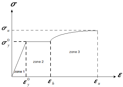
Figure 6.1.1-a : Behavior curve.
6.1.2. Cyclic loading#
We now consider the case where the bar undergoes a discharge following the first load. Two cases then arise:
the starting position is located in the elastic zone. In this case, the discharge remains elastic,
the starting position is located in the plastic zone (\(\varepsilon \ge {\varepsilon }_{y}^{0}\)). The response is first elastic, then, for a certain value of the deformation, the discharge becomes non-linear [Figure] (this is true for a discharge from zone 2 or zone 3).
The relationship that the deformation must satisfy in order for the Giuffré curve to be activated is as follows:
\(∣{\varepsilon }_{\mathrm{max}}-\varepsilon ∣>\frac{∣{\varepsilon }_{y}^{0}∣}{3.0}\), with \({\varepsilon }_{\mathrm{max}}\) the maximum deformation achieved under load.
As soon as this limit is crossed at the first discharge, cyclical behavior (Giuffré curve [Figure]) is activated.
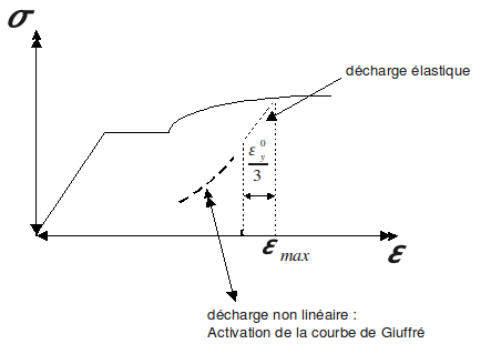
Figure 6.1.2-a : Behavior curve with discharge.
6.1.2.1. Presentation of the n-th half-cycle#
The shape of the curve of the n-th half-cycle depends on the plastic excursion carried out during the preceding half-cycle. The following quantities are defined [Figure]:
\({\sigma }_{y}^{n}\): Elastic limit of the n-th half-cycle. (Calculation explained in [§5.1.2.2])
\({\sigma }_{r}^{n-1}\): Stress at the last reversal point (maximum stress reached at the n-1st half-cycle).
\({\varepsilon }_{r}^{n-1}\): Deformation at the last point of reversal (maximum deformation reached at the n-1st half-cycle).
\({\varepsilon }_{y}^{n}\): Deformation corresponding to \({\sigma }_{y}^{n}\): \({\varepsilon }_{y}^{n}={\varepsilon }_{r}^{n-1}+\frac{{\sigma }_{y}^{n}-{\sigma }_{r}^{n-1}}{E}\)
\(f(t)\): Plastic excursion of the n-th cycle
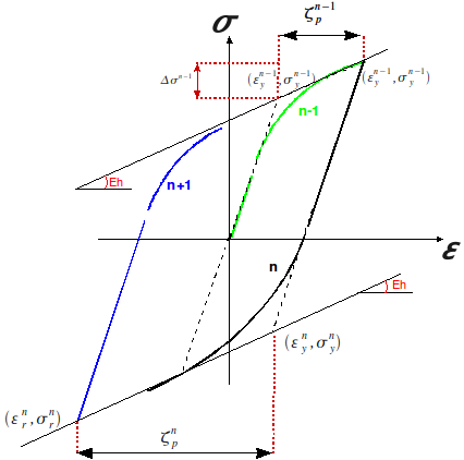
Figure 6.1.2.1-a : Cyclic behavior.
6.1.2.2. Work hardening law#
The model is based on a kinematic work-hardening law. The branches of the half-cycles are between two asymptotes with slope \({E}_{h}\) (asymptotic work-hardening slope).
We therefore determine \({\sigma }_{y}^{n}\) in the following way: \({\sigma }_{y}^{n}={\sigma }_{y}^{n-1}\mathrm{.}\mathrm{sign}(-{\zeta }_{p}^{n-1})+\Delta {\sigma }^{n-1}\) where the function \(\mathrm{sign}(x)=-1\) if \(x<0\) and \(1\) if \(x>0\) and where \(\Delta {\sigma }^{n-1}\) is the plastic stress increment of the previous half-cycle [Figure] which is defined by: \(\Delta {\sigma }^{n-1}={E}_{h}{\zeta }_{p}^{n-1}\).
For each half-cycle we therefore determine \({\sigma }_{y}^{n}\) as a function of \({\sigma }_{y}^{n-1}\) and \({\zeta }_{p}^{n-1}\), we deduce, \({\varepsilon }_{y}^{n}\) and then we calculate the next half-cycle (by the law of behavior below). The maximum deformation (in absolute value) reached before changing direction will allow the plastic excursion \({\zeta }_{p}^{n}={\varepsilon }_{r}^{n}-{\varepsilon }_{y}^{n}\) to be calculated.
6.1.2.3. Analytical description of curves \(\sigma =f(\varepsilon )\)#
The expression chosen in the model to describe the loading curves is as follows:
\({\sigma }^{\text{*}}=b{\varepsilon }^{\text{*}}+(\frac{1-b}{{(1+{({\varepsilon }^{\text{*}})}^{R})}^{1/R}}){\varepsilon }^{\text{*}}\)
With \(b=\frac{{E}_{h}}{E}\) ratio of the work-hardening slope to the elasticity slope.
\(\begin{array}{}{\varepsilon }^{\text{*}}=\frac{\varepsilon -{\varepsilon }_{r}^{n-1}}{{\varepsilon }_{y}^{n}-{\varepsilon }_{r}^{n-1}}\\ {\sigma }^{\text{*}}=\frac{\sigma -{\sigma }_{r}^{n-1}}{{\sigma }_{y}^{n}-{\sigma }_{r}^{n-1}}\\ {\xi }_{p}^{n-1}=\frac{{\zeta }_{p}^{n-1}}{{\varepsilon }_{y}^{n}-{\varepsilon }_{r}^{n-1}}\end{array}\)
The quantity \(R\) allows you to describe the shape of the curvature of the branches. It is a function of the plastic path carried out during the previous half-cycle:
\(R(\xi )={R}_{0}-g(\xi )\) where \(g(\xi )=\frac{{A}_{1}\mathrm{.}\xi }{{A}_{2}+\xi }\)
The parameters \({R}_{0},{A}_{1}\) and \({A}_{2}\) are unitless constants that depend on the mechanical properties of the steel. Their values are obtained experimentally and Menegotto [bib] proposes:
\({R}_{0}=20.0{A}_{1}=18.5{A}_{2}=.015\)
6.1.3. Case of inelastic buckling#
Monti and Nuti [bib] show that for a ratio between the length \(L\) and the diameter \(D\) of the bar that is less than 5, the compression curve is identical to that of tension. On the other hand, when \(L/D>5\) we observe a buckling of the bar. In this case, the compression curve in the plastic zone has a softening behavior. The model available in*Code_Aster* also makes it possible to describe this phenomenon.
The following variables are defined [Figure]:
\({E}_{0}\): Initial elastic Young’s modulus (corresponding to E without buckling).
\({b}_{c}\): Ratio of the work-hardening slope to the elastic slope under compression.
\({b}_{t}\): Ratio of the work-hardening slope to the elastic slope under tension (recharge after compression with buckling).
\({E}_{r}\): Reduced Young’s modulus in traction (slope of the recharge curve after compression with buckling).
Figure 6.1.3-a : Cyclic behavior curve.
6.1.3.1. Compression#
A negative slope \({b}_{c}\times E\) is introduced, where \({b}_{c}\) is defined by:
\({b}_{c}=a(5.0-L/D)e(b\zeta \text{'}\frac{E}{{\sigma }_{y}^{0}-{\sigma }^{\infty }})\)
With \({\sigma }_{\infty }=4.0\frac{{\sigma }_{y}^{0}}{L/D}\) and \(\zeta \text{'}=\mathrm{max}(∣{\zeta }_{p}^{n}∣)\) the longest plastic journey made during loading.
Next, as in the model without buckling, we must determine \({\sigma }_{y}^{n}\). The method is identical, but an additional constraint \({\sigma }_{s}^{\text{*}}\) is added in order to correctly position the curve in relation to the asymptote [Figure].
\({\sigma }_{s}^{\text{*}}={\gamma }_{s}bE\frac{b-{b}_{c}}{1-{b}_{c}}\) where \({\gamma }_{s}\) is given by: \({\gamma }_{s}=\frac{11.0-L/D}{10({e}^{\mathrm{cL}/D}-1.0)}\)
And so we have: \({\sigma }_{y}^{n}={({\sigma }_{y}^{n})}_{\text{sans flambage}}+{\sigma }_{s}^{\text{*}}\)
This also changes the value of \({\varepsilon }_{y}^{n}={\varepsilon }_{r}^{n-1}+\frac{{\sigma }_{y}^{n}\ast {\sigma }_{r}^{n-1}}{E}\)
6.1.3.2. Traction#
During the following traction half-cycle, a reduced Young’s modulus is adopted, defined by:
\({E}_{r}={E}_{0}({a}_{5}+(1.0-{a}_{5}){e}^{(-{a}_{6}{\zeta }_{p}^{2})})\) with \({a}_{5}=1.0+(5.0-L/D)/7.5\)
Note:
The parameters \(a,c\) and \({a}_{6}\) are constants (without units) depending on the mechanical properties of steel and are determined experimentally. The values adopted by Monti and Nuti [bib ] are: \(a=0.006c=0.500{a}_{6}=620.0\)
6.2. Implementation in Code_Aster#
This model can be accessed in Code_Aster using the keyword COMPORTEMENT (RELATION =” PINTO_MENEGOTTO “) or (RELATION =” GRILLE_PINTO_MEN”) from the STAT_NON_LINE [U4.51.03] command. All the parameters of the model are given via the command DEFI_MATERIAU (keyword factor PINTO_MENEGOTTO) [U4.43.01]. The parameters used in the model are listed here:
Model parameters |
Occurs in |
value adopted by default in Aster |
\({\sigma }_{y}^{0}\) |
First load |
_ |
\({\varepsilon }_{u}\) |
First load |
_ |
\({\sigma }_{u}\) |
First load |
_ |
\({\varepsilon }_{h}\) |
First load |
_ |
\(b=\frac{{E}_{h}}{E}\) |
Cycles |
If no value is entered we take the value calculated at the first load |
\({R}_{0}\) |
Cycles |
20 |
\({a}_{1}\) |
Cycles |
18.5 |
\({a}_{2}\) |
Cycles |
0.15 |
\(L/D\) |
Cycles with buckling (if \(L/D>5\)) |
4 (to be by default excluding buckling) |
\({a}_{6}\) |
Flambage |
620 |
\(c\) |
Flambage |
0.5 |
\(a\) |
Buckling |
0.006 |
The parameters \({R}_{0},{a}_{1},{a}_{2},{a}_{6},c\) and \(a\) depend on the mechanical properties of the steel and are determined experimentally. The values adopted by default in*Code_Aster* are those proposed in the literature [bib].
In [Figure] we give a comparison of the model according to the value of \(b=\frac{{E}_{h}}{E}\) for two values: \(b=0.01\) and \(b=0.001\)
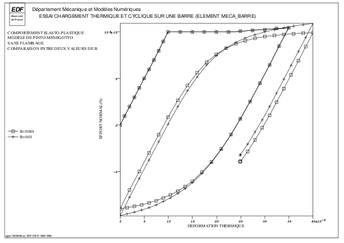
Figure 6.2-a : Comparison of 2 sets of parameters.
A comparison of the model without buckling and the model with buckling is given in [Figure].
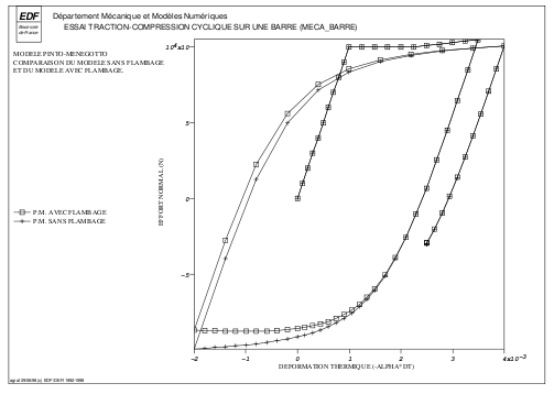
Figure 6.2-b : Comparison with and without buckling.
6.3. Internal variables#
They are 8 in number, and defined by:
\(\begin{array}{c}V1={\mathrm{\epsilon }}_{r}^{n-1}\phantom{\rule{2em}{0ex}};\phantom{\rule{2em}{0ex}}V2=\mathrm{\epsilon }{,}_{r}^{n}\phantom{\rule{2em}{0ex}};\phantom{\rule{2em}{0ex}}V3={\mathrm{\sigma }}_{r}^{n}\phantom{\rule{2em}{0ex}};\phantom{\rule{2em}{0ex}}V4={\mathrm{\epsilon }}^{\text{-}}+\mathrm{\Delta }\mathrm{\epsilon }-\mathrm{\alpha }\left(T-{T}^{\text{-}}\right)\phantom{\rule{2em}{0ex}};\phantom{\rule{2em}{0ex}}V5=\mathrm{\Delta }\mathrm{\epsilon }+\mathrm{\alpha }\left(T-{T}^{\text{-}}\right)\hfill \\ \begin{array}{cc}V6=\text{cycl}& \text{=}\phantom{\rule{2em}{0ex}}0\text{si le comportement cyclique n'est pas activé}\\ \text{}& \text{=}\phantom{\rule{2em}{0ex}}\text{1 dans le cas contraire}\\ V7=\mathrm{\chi }& \text{=}\phantom{\rule{2em}{0ex}}\text{0 si le pas de temps correspond à une évolution linéaire}\\ \text{}& \text{=}\phantom{\rule{2em}{0ex}}\text{1 dans le cas contraire (indicateur de plasticité}\\ V8=\text{indicateur de flambage}& \text{}\end{array}\hfill \end{array}\)