4. Linear search#
The linear search presented here concerns linear research in the absence of control.
4.1. Principle#
The introduction of linear search in operator STAT_NON_LINE is the result of an observation: the Newton method with a consistent matrix does not converge in all cases, especially when one starts too far from the solution. On the other hand, the use of matrices other than the consistent tangent matrix can, when they are too « soft », lead to divergence. Linear research makes it possible to avoid such discrepancies.
It consists in considering \((\delta {u}_{i}^{n},\delta {\lambda }_{i}^{n})\), no longer as the increment of movements and Lagrange multipliers, but as a direction of research in which we will try to minimize a functional (the energy of the structure). We will find a \(\rho\) step forward in this direction, and updating the unknowns will consist in doing:
In the absence of a linear search (by default) the scalar \(\rho\) is of course equal to 1.
4.2. Minimization of a functional#
In order to better convince ourselves of the validity of linear research, we can interpret Newton’s method as a method of minimizing a functional (in the case where the tangent matrices are symmetric). We emphasize the fact that the equations obtained are rigorously those of Newton’s method set out in [§ 2] and that only the way to achieve them is different.
To simplify the explanation, « Let’s forget » the dualization of the conditions at the Dirichlet limits and put ourselves into the hypothesis of small deformations. We consider the functional:
: label: eq-125
begin {array} {} J:Vto ↓\ uto J (u) = {int} _ {Omega}Phi (varepsilon (u))mathrm {.} domega - {int} - {int} _ {int} _ {int} _ {int} _ {int} _ {int} _ {int} _ {gamma} _ {Gamma} tmathrm {.} umathrm {.} dGammaend {array}
where the free energy density \(\Phi\) makes it possible to connect the stress tensor \(\sigma\) to the linearized deformation tensor \(\varepsilon\) by the relationship \(\varepsilon =\frac{\partial \Phi }{\partial \sigma }\) in the case of hyperelasticity (this situation is generalized to the other nonlinearities in the rest of the document). Since functional \(J\) is convex, finding the minimum of \(J\) is equivalent to cancelling its gradient, i.e.:
This is exactly the Principle of Virtual Works since:
: label: eq-127
nabla J (u)mathrm {.} v= {int} _ {int} _ {omega}sigma (u):varepsilon (v)mathrm {.} domega - {int} _ {int} _ {int} _ {int} _ {int} _ {int} _ {int} _ {int} _ {int} _ {int} _ {int} _ {int} _ {int} _ {int} _ {int} _ {int} _ {int} _ {int} _ {int} _ {int} _ {int} _ {int} _ {int} _ {int} _ {int} _ {int} _ {int} _.} vmathrm {.} dGamma
Thus, solving the equations from the Principle of Virtual Works (basis of the problem formulated in [§ 1.3]) is equivalent to minimizing the functional \(J\) which represents the energy of the structure (internal energy reduced by the work of external forces \(\mathrm{f}\) and \(t\)).
4.3. Minimization method#
Minimization is done iteratively, classically in two stages at each iteration:
Calculation of a search direction \(\delta\) along which we will search for the next iteration,
Calculation of the best step forward \(\rho\) in this direction: \({u}^{n+1}={u}^{n}+\rho \text{.}\delta\)
In a minimization problem, the natural idea is to advance in the direction opposite to the functional gradient, which is locally the best direction of descent since this direction is normal to the isovalue lines and directed in the direction of decreasing values Figure 2-4.3-1
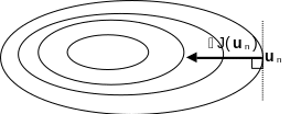
Figure 2 ‑ 4.3-1
However, it is possible to improve the choice of descent direction by using this gradient method in a new metric. This is what will allow us to find the classical equations of Newton’s method. Let’s take the simple example of a problem with two variables \(x\) and \(y\) for which the functional has the shape of an ellipse whose minimum is in \((\frac{\alpha }{a},\frac{\beta }{b})\):
By choosing the inverse of the \(J\) gradient as the direction of descent, we go from one iterate to the next (let’s reason on \(x\) only) by:
: label: eq-129
{x} ^ {n+1} = {x} ^ {n} - {text {ax}} ^ {n} +alpha
which does not point to the solution since the normal at a point in an ellipse does not generally pass through the center of the ellipse
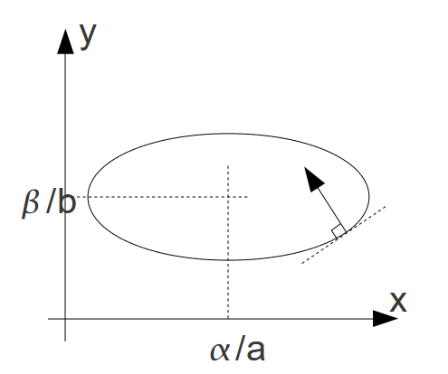
Figure 2‑ 4.3-2
On the other hand, if we change the variables so that the isovalues of \(J\) become circles:
: label: eq-130
{begin {array} {}stackrel {} {x} =sqrt {a}mathrm {.} x\ stackrel {} {y} =sqrt {b}mathrm {.}mathrm {.} {x} =sqrt {b}\mathrm {.} {x} =sqrt {b}\\ mathrm {.} {x} =sqrt {b}\mathrm {.} {.} y\stackrel {} {y} =sqrt {b}\mathrm {.} {.} y\stackrel {} {y} =sqrt {b}\mathrm {.} {y}) =frac {1} {2}mathrm {.} ({stackrel {} {x}}} ^ {2}} + {stackrel {} {y}} ^ {2}) -frac {alpha} {sqrt {a}} {sqrt {a}}mathrm {.} stackrel {} {x} -frac {beta} {sqrt {b}}mathrm {.} stackrel {} {y}end {array}
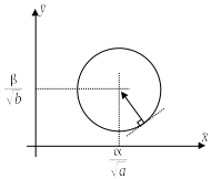
Figure 2 ‑ 4.3-3
The use of the inverse direction of the \(\stackrel{ˉ}{J}\) gradient then makes it possible to obtain the solution in one iteration:
: label: eq-131
{stackrel {} {x}}} ^ {n+1}mathrm {=} {stackrel {} {x}}} ^ {n}mathrm {-} ({stackrel {} {} {x} {x}} {x}}} ^ {x}} ^ {n}} ^ {n}}mathrm {-}}mathrm {-})mathrm {-} ({stackrel {}} {x}} ({stackrel {}} {x}} ({stackrel {}} {x}} ({stackrel {}} {x}} ({stackrel {}} {x}} ({stackrel {} {frac {alpha} {sqrt {a}}}mathrm {Rightarrow} {x} ^ {n+1}mathrm {=}frac {alpha} {a}
Thus, the use of the gradient method in the new metric allows for immediate convergence. In a more complicated case (functional convex but different from an ellipse), convergence is not instantaneous but the change of variables makes it possible to significantly reduce the number of iterations required.
4.4. Application to the minimization of energy#
To simplify, we will place ourselves in the discretized linear case where the functional \(J\) is equal to:
: label: eq-132
J (u) =frac {1} {2}mathrm {.} {u} ^ {T}mathrm {.} Kmathrm {.} u- {u} ^ {T}mathrm {.} L
We note \(K\) the stiffness matrix of the structure, and \(L\) the vector of imposed loads. To minimize \(J\) , we will use the same descent method as before by making a completely similar change of variables beforehand. Since the matrix \(K\) is symmetric definite positive, its eigenvalues are real positive: we can therefore define the « square root » of \(K\) which will be denoted by \(\sqrt{K}\) (also symmetric). We set \(\stackrel{ˉ}{u}=\sqrt{K}\mathrm{.}u\), the minimization of \(J\) is then equivalent to that of:
: label: eq-133
stackrel {} {J} (stackrel {}} {mathrm {u}})mathrm {=}frac {1} {2}mathrm {.} {stackrel {} {mathrm {u}}}} ^ {T}mathrm {.} stackrel {} {mathrm {u}}mathrm {-} {stackrel {} {mathrm {u}}}} ^ {T}mathrm {.} {(sqrt {mathrm {K}}})}}} ^ {mathrm {-} T}mathrm {.} mathrm {L}
Using a diagonal decomposition:
With \(\mathrm{D}\) diagonal, so:
Which leads to:
Taking the opposite direction of the \(\stackrel{ˉ}{J}\) gradient as the direction of descent, we obtain:
Or, going back to the initial variables:
: label: eq-138
{u} ^ {n+1} = {u} ^ {n} - {K} ^ {-1}mathrm {.} (Kmathrm {.} {u} ^ {n} -L)
Or even:
We find the equations of Newton’s method: the \(K\) matrix is the Hessian of the functional \(J\) (second derivative matrix) and the second member is the difference in loading and internal forces, also called the equilibrium residue. Thus Newton’s method can be interpreted as resulting from the minimization of the energy of the structure via a gradient method applied after a change in metric.
4.5. Determining the progress step#
Let’s get back to the real problem, that of solving \({L}_{i}^{\text{int}}({u}_{i})={L}_{i}^{\text{ext}}\). This problem can be interpreted as the minimization of the following functional:
where \(W({u}_{i})\) corresponds to the discretization, based on form functions, of the internal energy of the structure:
: label: eq-141
W= {int} _ {omega}Phi (varepsilon (u))mathrm {.} dOmega
A displacement increment \(\delta {u}_{i}^{n}\) was calculated by Newton’s method, which, in the minimization problem, is interpreted as a search direction, based on the above. We will calculate the progress step \(\rho\) in this direction to minimize the value of the functional:
: label: eq-142
underset {rhoin ↓} {text {Min}} {text {Min}}}left{W ({u} _ {i} ^ {n-1}} +rhomathrm {.} delta {u} _ {i} ^ {n}) - {L} _ {n}) - {L} _ {n}) - {L} _ {i} ^ {n-1}) +rhomathrm {.} delta {u} _ {i} ^ {n})right}
To find the minimum of this scalar function of \(\rho\), which we will note \(f(\rho )\), we look for the point where its derivative is cancelled out (this is equivalent to making the final residue and the search direction orthogonal):
\(f\text{'}(\rho )\) is the projection of the residue onto the research direction. With the notations of [§ 2.2] and taking into account the support reactions, the scalar equation to be solved to determine the progress step \(\rho\), is written:
: label: eq-144
ftext {”} (rho) = {left [delta {u} _ {i} ^ {n}right]} ^ {T}mathrm {.} left [{Q} ^ {T}mathrm {.} sigma ({u} _ {i} ^ {n-1} +rhomathrm {.} delta {u} _ {i} ^ {n}) + {B} ^ {T}mathrm {.} ({lambda} _ {i} ^ {n-1} +rhomathrm {.} delta {lambda} _ {i} ^ {n}) - {L} _ {i} ^ {text {ext}}right] =0
At the end of the linear search, the Lagrange movements and parameters are updated by:
: label: eq-145
{begin {array} {c} {mathrm {u}}} _ {i} ^ {n} = {mathrm {u}} _ {i} ^ {n-1} +rhomathrm {.} delta {mathrm {u}} _ {i} ^ {n} ^ {n}\ {lambda} _ {i} ^ {n} = {lambda} _ {i} ^ {n-1} +rhomathrm {.} delta {lambda} _ {i} ^ {n}end {array}
The convergence test covers:
On the maximum number of linear search iterations indicated by the user under the keyword ITER_LINE_MAXI of the keyword factor NEWTON (the default value 0 inhibits linear search, and \(\rho\) then equals 1),
On the criterion RESI_LINE_RELA given by \(f(\rho )\le \tau \text{.}f(0)\), where \(\tau\) is 0.1 by default.
Linear research is in a sense an « insurance » to protect against serious discrepancies in Newton’s method. When the search direction is « bad » (if the tangent matrix is too soft, for example), the linear search algorithm results in a low value of \(\rho\), which prevents straying too far from the solution. It is not necessary to do a lot of iterations in the secant method (two or three are enough to avoid catastrophes) because each one is quite expensive (you have to recalculate the internal forces) and we do not have the ambition to find at each Newton’s iteration the truly optimal value of \(\rho\).
4.6. Calculation of the linear search coefficient#
There are two methods for calculating the optimal \(\rho\) in linear search*.*
4.6.1. Secant method (METHODE =” CORDE “)#
In order for the determination of \(\rho\) not to be too expensive, a secant method is used whose maximum number of iterations is set by the user. The secant method can be interpreted as a Newton method where the derivative at the current point is approximated by the direction joining the current point and the previous point:
Where we noted \({g}^{p}=f\text{'}({\rho }^{p})\). We’re starting from \({\rho }^{0}\mathrm{=}0\) and \({\rho }^{1}=1\). The secant method has an order of convergence in the order of 1.6. It is shown schematically on the Figure 2-4.6.1-1.
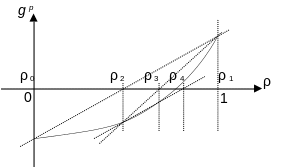
Figure 2 ‑ 4.6.1-1
4.6.2. Mixed method (METHODE =” MIXTE “)#
This method combines several resolution techniques to be more robust. It consists essentially in the application of a secant method (see previous paragraph) between two pre-determined limits. It is in fact the application of the secant method with variable limits. Here is the algorithm used:
Assume \(f\text{'}(0)>0\). If this is not the case, we change the direction of the descent (by examining negative \(\rho\)), which is the same as defining \(f\text{'}\) as being equal to \(-f\text{'}\).
We’re looking for a positive \({\rho }_{\text{max}}\) like \(f\text{'}({\rho }_{\text{max}})<0\). The method is simply iterative by doing \({\rho }_{n+1}=3\text{.}{\rho }_{n}\) with \({\rho }_{0}=1\) (bracketing or framing step)
We thus have the two new limits between which the function changes sign. If we assume that function \(f\text{'}\) is continuous, there is therefore a solution between these limits.
We apply the secant method on this interval: we start from \({\rho }^{0}=0\) and \({\rho }^{1}={\rho }_{\mathrm{max}}\).
4.6.3. Special case: the Newton-Krylov method#
It was specified above that the linear search is carried out simultaneously on the unknowns \(\mathrm{u}\) and \(\lambda\) as shown by the formula () for updating the variables. However, the functional to be minimized does not have a minimum according to the unknowns \((\mathrm{u},\lambda )\), it is in fact a Lagrangian who has a saddle point, that is to say a minimum in \(\mathrm{u}\) and a maximum in \(\lambda\) (see [R3.03.01]). This way of doing things is therefore not legal in the general case.
That said, it can be shown that in the case where the prediction system is solved « exactly » (at least to a numerically satisfactory precision), this approach is legitimate. This is generally the case in the usual use of*Code_Aster*.
However, this is not the case when using the Newton-Krylov method, where linear systems are precisely resolved in a deliberately inaccurate manner. In this situation, to get around the problem, only the unknowns \(\mathrm{u}\) are affected by the linear search and the formula for updating the variables therefore becomes:
: label: eq-147
{begin {array} {c} {mathrm {u}}} _ {i} ^ {n} = {mathrm {u}} _ {i} ^ {n-1} +mathrm {n-1} +mathrm {n-1} +mathrm {n-1} +mathrm {n-1} +mathrm {n-1} +mathrm {rho}mathrm {.} mathrm {delta} {mathrm {u}}} _ {i}} _ {i}} ^ {n}\ mathrm {lambda}} _ {i} ^ {n} = {mathrm {lambda}}} _ {lambda}}} _ {mathrm {lambda}} = {mathrm {lambda}} = {mathrm {lambda}} = {mathrm {lambda}} = {mathrm {lambda}} = {mathrm {lambda}} = {mathrm {lambda}} = {mathrm {lambda}} = {mathrm {lambda}} = {mathrm {lambda}end {array}
Insofar as the functional to be minimized has a minimum in \(\mathrm{u}\), the linear search procedure is legal.
Insofar as the functional to be minimized has a minimum in \(\mathrm{u}\), the linear search procedure is legal.