3. Principle of virtual work

3.1. Deformation work

The general expression of 3D deformation work for a plate is as follows:

(3.1)\[ {W} _ {\ text {def}} =\ underset {S} {\ s} {\ int} {\ int}\ underset {-h/2} {\ int}} ({\ varepsilon}} _ {\ text {xx}} {\ text {xx}}} {\ text {xx}}} {\ sigma} _ {\ text {yy}}} {\ sigma} _ {\ text {yy}}} {\ sigma} _ {\ text {yy}}} {\ sigma} _ {\ text {yy}}} {\ sigma} _ {\ text {yy}}} {\ sigma} _ {\ text {yy}}} {\ sigma} _ {\ text {yy}}} {\ sigma} _ {\ text {yy}}} {\ sigma} _ {\ text {{\ text {yy}} + {\ gamma} _ {\ text {xy}} {\ text {xy}}} {\ sigma} _ {\ gamma} _ {\ sigma} _ {\ sigma} _ {\ text {xz}} _ {\ text {xz}}}} + {\ gamma}}} + {\ gamma}}} + {\ text {xz}} _ {\ gamma}} _ {\ gamma}} _ {\ gamma} _ {\ sigma}})\ text {xz}} _ {\ text {xz}} _ {\ text {xz}} _ {\ text {xz}} _ {\ text {xz}} _ {\ text {xz}}\]

where \(S\) is the mean area and the position in the thickness of the plate varies between \(–h\mathrm{/}2\) and \(+h\mathrm{/}2\).

3.1.1. Expression of the resulting efforts

By adopting the kinematics of §2.2.1, we identify the work of internal forces:

\({W}_{\text{def}}=\underset{S}{\int }({e}_{\text{xx}}{N}_{\text{xx}}+{e}_{\text{yy}}{N}_{\text{yy}}+2{e}_{\text{xy}}{N}_{\text{xy}}+{\kappa }_{\text{xx}}{M}_{\text{xx}}+{\kappa }_{\text{yy}}{M}_{\text{yy}}+2{\kappa }_{\text{xy}}{M}_{\text{xy}}+{\gamma }_{x}{T}_{x}+{\gamma }_{y}{T}_{y})\text{dS}\) where:

(3.2)\[\begin{split} N= (\ begin {array} {c} {N} _ {\ text {xx}} _ {\ text {xx}}}\\ {N}}\\ {N} _ {\ text {xy}}\ end {array}}\ end {array}) =\ underset {-h/2} {\ text {\ array}} {\ text {xy}}\ end {array}}\ end {array}}\ end {array}}\ end {array}}) =\ underset {-h/2} {\ text {xx}}\\ {\ sigma} _ {\ text {yy}}}\\ {\ sigma} _ {\ text {xy}}\ end {array})\ text {yy})\ text {dz}\end{split}\]

\({N}_{\text{xx}},{N}_{\text{yy}},{N}_{\text{xy}}\) are the resulting membrane stresses (in \(N\mathrm{/}m\));

\({M}_{\text{xx}},{M}_{\text{yy}},{M}_{\text{xy}}\) are the resulting flexural forces or moments (in \(N\));

\({T}_{x},{T}_{y}\) are the resulting shear forces or shear forces (in \(N\mathrm{/}m\)).

3.1.2. Relationship between resultant forces and deformations

The expression deformation work is also written:

(3.3)\[ {W} _ {\ text {def}}\ mathrm {=}\ underset {s} {\ mathrm {\ int}}\ underset {\ mathrm {-} h\ mathrm {/} 2} {\ mathrm {/} 2} {\ mathrm {\ int}}}\ mathrm {[}\ varepsilon\ text {C} (e,\ alpha)\ varepsilon\ mathrm {]}\ text {dV}\ mathrm {=}\ underset {s} {\ mathrm {\ int}}\ underset {\ mathrm}}}\ underset {\ mathrm {-} -} h\ mathrm {-} h\ mathrm {-} h\ mathrm {/} 2} {\ mathrm {-} h\ mathrm {-} h\ mathrm {/} 2} {\ mathrm {\ int}}}\ mathrm {[}\ text {ECe} +z\ text {eC} +z\ text {eC}\ kappa\ text {Ce} + {z} ^ {2}\ kappa\ text {C}\ text {C}\ kappa +\ gamma\ text {EC}\ gamma\ mathrm {]}\ text {dV}\]

where \(\text{C}(e,\alpha )\) is the local behavior matrix.

Using the expression obtained for \({W}_{\text{def}}\) in the previous paragraph we find the following relationship between the resulting forces and the deformations:

(3.4)\[\begin{split} \ begin {array} {c}\ text {N} = {\ text {H}} = {\ text {H}} = {\ text {H}} _ {\ text {mf}}\ mathrm {\ kappa}\\ kappa}\\\ text {M} = {\ text {M}} = {\ text {H}}} _ {f} = {\ text {H}}} _ {f}\ mathrm {\ kappa}\\\ text {T} = {\ text {H}} _ {\ text {ct}}\ mathrm {\ gamma}\ end {array}\ end {array}\end{split}\]

where:

\({H}_{\text{ct}}=\left(\begin{array}{cc}{G}_{\text{11}}& 0\\ 0& {G}_{\text{22}}\end{array}\right)\) \(\text{e}=\left(\begin{array}{c}{e}_{\text{xx}}\\ {e}_{\text{yy}}\\ 2{e}_{\text{xy}}\end{array}\right),\mathrm{\kappa }=\left(\begin{array}{c}{\mathrm{\kappa }}_{\text{xx}}\\ {\mathrm{\kappa }}_{\text{yy}}\\ 2{\mathrm{\kappa }}_{\text{xy}}\end{array}\right),\mathrm{\gamma }=\left(\begin{array}{c}{\mathrm{\gamma }}_{x}\\ {\mathrm{\gamma }}_{y}\end{array}\right)\)

Matrixes \({\text{H}}_{m},{\text{H}}_{f}\text{et}{\text{H}}_{\text{ct}}\) are the matrices for membrane stiffness, flexure, and transverse shear, respectively. Matrix \({\text{H}}_{\text{mf}}\) is a matrix of coupling stiffness between the membrane and the flexure.

For an isotropic homogeneous elastic behavior of plates, these matrices have the following expressions:

(3.5)\[\begin{split} {\ text {H}} _ {m} =\ frac {\ text {Eh}} {1- {v} ^ {2}}\ left (\ begin {array} {ccc} 1& v& 0\\ v& 1& 1& 0\\ v& 1& 0\\ 0& 0\\ 0&\ 0&\ frac {1-v} {2}}\ end {array}\ right), {\ text {H}}} {ccc} 1& v& 0\\ v& 1& 0\\ v& 1& 0\\ 0& 0\\ 0& 0&\ frac {1-v} {2}}\ end {array}\ right), {\ text {H}}} _ {f} =\ frac {{\ text {Eh}} ^ {3}} {\ text {3}}} {\ text {12}} (1- {v} ^ {2})}\ left (\ begin {array} {ccc} 1& v& 0\\ v& 1& 0\\ 0& 0\\ 0&\ 0&\ frac {1-v} {2}}\ left (\ begin {array} {ccc}} 1& v& 0\\ v& 1& 0\\ v& 1& 0\\ 0& 0\\ 0& 0&\ frac {1-v} {2}\ end {array}\ right), {\ text {H}}} _ {\ text {ct}}}} =\ frac {\ text {keH}}} {2 (1+v)}\ left (\ begin {array} {cc} 1& 0\\ 0& 1\ end {array}\ right)\end{split}\]

and \({\text{H}}_{\text{mf}}=0\) because there is material symmetry with respect to the \(z\mathrm{=}0\) plane.

For an orthotropic material, the behavior is given in the appendix.

3.1.3. Elastic internal energy of plate

Taking into account the preceding remarks, the elastic internal energy of the plate is more usually expressed for this type of geometry in the following way:

(3.6)\[ {\ mathrm {\ Phi}} _ {\ text {int}}} =\ frac {1} {2}\ underset {S} {\ int} [\ text {e} ({\ text {H}}} _ {m} _ {m}\ text {e}} + {\ text {e}} + {\ text {H}}} _ {\ text {\ kappa}}) +\ mathrm {\ kappa}) +\ mathrm {\ kappa}) +\ mathrm {\ kappa}) +\ mathrm {\ kappa}) +\ mathrm {\ kappa}) +\ mathrm {\ kappa}) +\ mathrm {\ kappa}) +\ mathrm {\ kappa}) +\ mathrm {appa} ({\ text {H}} _ {\ text {mf}}}\ text {e}}\ text {e}} + {\ text {H}} _ {f}\ mathrm {\ kappa}) +\ mathrm {\ gamma}} {\ gamma}}\ mathrm {\ gamma}}) +\ mathrm {\ gamma}}) +\ mathrm {\ gamma}}) +\ mathrm {\ gamma}}\ mathrm {\ gamma}}) +\ mathrm {\ gamma}} {\ gamma}}\ mathrm {\ gamma}}) +\ mathrm {\ gamma}} {\ gamma}}\ mathrm {\ gamma\]

which can be broken down as follows:

\({\mathrm{\Phi }}_{\text{membrane}}=\frac{1}{2}\underset{S}{\int }\text{e}{\text{H}}_{m}\text{e}\text{dS}\) membrane energy

\({\mathrm{\Phi }}_{\text{flexion}}=\frac{1}{2}\underset{S}{\int }\mathrm{\kappa }{\text{H}}_{m}\mathrm{\kappa }\text{dS}\) flexural energy

\({\mathrm{\Phi }}_{\text{cisaillement}}=\frac{1}{2}\underset{S}{\int }\mathrm{\gamma }{\text{H}}_{\mathit{ct}}\mathrm{\gamma }\text{dS}\) shear energy

\({\mathrm{\Phi }}_{\text{couplage}}=\frac{1}{2}\underset{S}{\int }(\text{e}{\text{H}}_{\text{mf}}\mathrm{\kappa }+\mathrm{\kappa }{\text{H}}_{\text{mf}}\text{e})\text{dS}\) membrane-flexure coupling energy

3.1.4. notes

The relationships linking \({\text{H}}_{m}\), \({\text{H}}_{f}\), \({\text{H}}_{\mathit{mf}}\) to \(\text{H}\) and \({\text{H}}_{\mathrm{ct}}\) to \({\text{H}}_{\gamma }\) are valid regardless of the law of behavior: elastic, with anelastic deformations (thermoelasticity, plasticity,…).

For a plate made up of \(N\) orthotropic layers in elasticity, the matrices \({\text{H}}_{m}\), \({\text{H}}_{f}\), \({\text{H}}_{\mathrm{mf}}\) and \({\text{H}}_{\mathit{ct}}\) are written:

(3.7)\[ {\ text {H}} _ {m} =\ sum _ {i=1} ^ {N} {h} _ {i} {\ text {H}} _ {i}, {\ text {H}}} _ {\ mathit {mf}} = {\ mathit {mf}}} =\ sum _ {i=1}} ^ {i=1} ^ {N} {h}} _ {i} {\ mathrm {\ eta}}} _ {i}} _ {i}} _ {i}} _ {i}} _ {i}} _ {i}} _ {i}} _ {i}} _ {i}} _ {i}} _ {i}} _ {i}} _ {i}} _ {i}} _ {i}} text {H}} _ {i}, {\ text {H}}} _ {f} =\ sum _ {i=1} ^ {N}\ frac {1} {3} ({z} _ {i+1}} ^ {3} ^ {3} ^ {3}) {\ text {H}} {3}) {\ text {H}} {3} ({z} _ {i+1}} ^ {3}} ^ {3}) {\ text {H}} {3} ({z} _ {i+1}} ^ {3}} ^ {3}) {\ text {H}}} _ {\ mathit {ct}} =\ sum _ {i=1} ^ {N} {h} {h} _ {i} {\ text {H}} _ {\ mathrm {\ gamma} i}\]

where: \({h}_{i}={z}_{i+1}-{z}_{i},{\mathrm{\eta }}_{i}=\frac{1}{2}\left({z}_{i+1}+{z}_{i}\right)\) and \({\text{H}}_{i},{\text{H}}_{\mathrm{\gamma }i}\) represent matrices \(\text{H}\) and \({\text{H}}_{\mathrm{\gamma }}\) for layer \(i\).

Homogenization for multilayer shells can lead to nonproportional membrane stiffness and flexure matrices of the type:

(3.8)\[\begin{split} {\ text {H}} _ {m} =\ left (\ begin {array} {ccc} {ccc} {C} _ {\ text {1111}} & {\ text {1122}}} & 0\\ {C}} _ {\ text {1122}} _ {\ text {1122}}} & {\ text {2222}} & {\ 0& 0& 0& {C}} & 0\\ {C}} _ {\ text {1222}} & 0\\ 0& {C}} _ {\ text {1222}} 12}}\ end {array}\ right), {\ text {H}}} _ {f} =\ left (\ begin {array} {ccc} {D} _ {\ text {1111}} & {D}} _ {\ text {1122}} _ {\ text {1122}}} & {\ text {1111}}} & {\ text {2222}} _ {\ text {2222}} _ {\ text {2222}} _ {\ text {2222}} _ {\ text {2222}}} & 0\\ 00 & 0& {D} _ {\ text {1212}}}\ end {array}\ right), {\ text {H}} _ {\ mathit {ct}} =\ left (\ begin {array} {cc} {CC} {G}}} _ {\ text {11}}} _ {\ text {22}} =\ left (\ begin {array} {CC} {G}} =\ left (\ begin {array} {CC} {G}} _ {\ text {22}}\ end {array} {G}} _ {\ text {22}}\ end {array} {G}} _ {\ text {22}}\ end {array}\ right)\end{split}\]

for which it is not possible to find equivalent values of the Young’s modulus and of the thickness making it possible to find the classical expressions of stiffness, cf. [4].

3.2. Work of forces and external couples

The work of the forces and torques exerted on the plate is expressed as follows:

(3.9)\[ {W} _ {\ text {ext}} =\ underset {S} {\ s} {\ int}\ underset {-h/2} {\ overset {+h/2} {\ int}} {\ int}}} {\ text {F}}} {\ text {F}}} {\ text {F}}} {\ text {F}}} {\ text {F}}} {\ text {F}}} _ {v}\ text {.} \ text {U}\ text {dV} +\ underset {S} {\ int} {\ text {F}} _ {s}\ text {.} \ text {U}\ text {dS} +\ underset {C} {\ C} {\ int}\ underset {-h/2} {\ overset {+h/2} {\ int}} {\ int}}} {\ text {F}}} {\ text {F}}} {\ text {F}}} {\ text {F}}} {\ text {F}}} _ {c}\ text {.} \ text {U}\ text {dz}\ text {ds}\]

where \({\text{F}}_{v},{\text{F}}_{s},{\text{F}}_{c}\) are the volume, surface, and contour forces exerted on the plate, respectively. \(C\) is the portion of the plate outline on which the \({\text{F}}_{c}\) contour forces are applied. With the kinematics in §2.2.1, we determine as follows:

\(\begin{array}{}{W}_{\text{ext}}=\underset{S}{\int }({f}_{x}u+{f}_{y}v+{f}_{z}w+{c}_{x}{\theta }_{x}+{c}_{y}{\theta }_{y})\text{dS}+\underset{C}{\int }({\phi }_{x}u+{\phi }_{y}v+{\phi }_{z}w+{\chi }_{x}{\theta }_{x}+{\chi }_{y}{\theta }_{y})\text{ds}\\ =\underset{S}{\int }({f}_{x}u+{f}_{y}v+{f}_{z}w+{c}_{y}{\beta }_{x}-{c}_{x}{\beta }_{y})\text{dS}+\underset{C}{\int }({\phi }_{x}u+{\phi }_{y}v+{\phi }_{z}w+{\chi }_{y}{\beta }_{x}-{\chi }_{x}{\beta }_{y})\text{ds}\end{array}\)

• where are present on the plate:

\({f}_{x},{f}_{y},{f}_{z}\): surface forces acting according to \(x,y\) and \(z\)

\({f}_{i}=\underset{-h/2}{\overset{+h/2}{\int }}{\text{F}}_{v}\text{.}{\text{e}}_{i}\text{dz}+{\text{F}}_{s}\text{.}{\text{e}}_{i}\) where \({\text{e}}_{x}\) and \({\text{e}}_{y}\) are the base vectors of the tangential plane and \({\text{e}}_{z}\) are their normal vector.

\({c}_{x},{c}_{y}\): surface couples acting around the \(x\) and \(y\) axes.

\({c}_{i}=\underset{-h/2}{\overset{+h/2}{\int }}(z{\text{e}}_{z}\wedge {\text{F}}_{v})\text{.}{\text{e}}_{i}\text{dz}+(\pm \frac{h}{2}{\text{e}}_{z}\wedge {\text{F}}_{s})\text{.}{\text{e}}_{i}\) where \({\text{e}}_{x},{\text{e}}_{y},{\text{e}}_{z}\) are the base vectors previously defined.

• and where are present on the outline of the plate:

\({\phi }_{x},{\phi }_{y},{\phi }_{z}\): linear forces acting according to \(x,y\) and \(z\)

\({\mathrm{\varphi }}_{i}=\underset{-h/2}{\overset{+h/2}{\int }}{\text{F}}_{c}\text{.}{\text{e}}_{i}\text{dz}\) where \({\text{e}}_{x},{\text{e}}_{y},{\text{e}}_{z}\) are the base vectors previously defined.

\({\mathrm{\chi }}_{x},{\mathrm{\chi }}_{y}\): linear torques around the \(x\) and \(y\) axes.

\({\mathrm{\chi }}_{i}=\underset{-h/2}{\overset{+h/2}{\int }}(z{\text{e}}_{z}\wedge {\text{F}}_{c})\text{.}{\text{e}}_{i}\text{dz}\) where \({\text{e}}_{x},{\text{e}}_{y},{\text{e}}_{z}\) are the base vectors previously defined.

Note:

The moments compared to \(z\) are zero.

3.3. Principle of virtual work

It is written as follows: \(\mathrm{\delta }{W}_{\text{ext}}=\mathrm{\delta }{W}_{\text{def}}\) for all kinematically eligible virtual movements and rotations.

3.3.1. Hencky cutscene

With this kinematics, after integration by parts of the deformation work, the following equations of static equilibrium for the plates are obtained:

• For the efforts: \(\begin{array}{}{N}_{\text{xx},x}+{N}_{\text{xy},y}+{f}_{x}=\mathrm{0,}\\ {N}_{\text{yy},y}+{N}_{\text{xy},x}+{f}_{y}=\mathrm{0,}\\ {T}_{x,x}+{T}_{y,y}+{f}_{z}=0\text{.}\end{array}\)

• For couples: \(\begin{array}{}{M}_{\text{xx},x}+{M}_{\text{xy},y}-{T}_{x}+{c}_{y}=\mathrm{0,}\\ {M}_{\text{yy},y}+{M}_{\text{xy},x}-{T}_{y}-{c}_{x}=0\text{.}\end{array}\)

as well as the following boundary conditions on contour \(C\) of \(S\):

\(\begin{array}{}{N}_{\text{xx}}{n}_{x}+{N}_{\text{xy}}{n}_{y}={\phi }_{x}\\ {N}_{\text{yy}}{n}_{y}+{N}_{\text{xy}}{n}_{x}={\phi }_{y}\\ {T}_{x}{n}_{x}+{T}_{y}{n}_{y}={\phi }_{z},\\ {M}_{\text{xx}}{n}_{x}+{M}_{\text{xy}}{n}_{y}={\chi }_{y}\\ {M}_{\text{yy}}{n}_{y}+{M}_{\text{xy}}{n}_{x}=-{\chi }_{x}\end{array}\) where \(\begin{array}{}u=\stackrel{ˉ}{u}\\ v=\stackrel{ˉ}{v}\\ w=\stackrel{ˉ}{w}\\ {\beta }_{x}={\stackrel{ˉ}{\theta }}_{y}\\ {\beta }_{y}=-{\stackrel{ˉ}{\theta }}_{x}\end{array}\)

where \({n}_{x}\) and \({n}_{y}\) are the direction cosines of the normal to \(C\) directed to the outside of the plate.and \(\overline{u}\) refers to the trace of \(u\) on C \(\mathrm{.}\)

The physical interpretation of these efforts (\(N\), \(T\), and \(M\)) based on the preceding equations is given below:

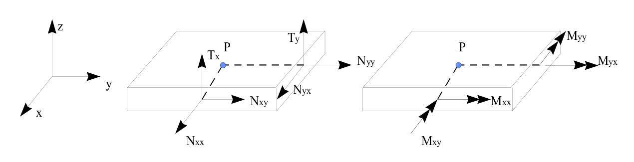
Figure 3.3.1-a: Resulting efforts for a plate element

Note:

\({N}_{\text{xx}},{N}_{\text{yy}}\) represent the tensile forces and \({N}_{\text{xy}}\) the plane shear. \({M}_{\text{xx}}\) and \({M}_{\text{yy}}\) represent the bending torques \({M}_{\text{xy}}\) the torsional torque. \({T}_{x}\) and \({T}_{y}\) are the transverse shear forces.

3.3.2. Love-Kirchhoff kinematics

We recall that in the context of this kinematics, we have the following relationship linking the derivative of the arrow to the rotations: \(\begin{array}{}{\beta }_{x}=-\frac{\partial w}{\partial x}\\ {\beta }_{y}=-\frac{\partial w}{\partial y}\end{array}\). After a double integration by parts of the deformation work, the following static equilibrium equations are obtained:

• For membrane efforts: \(\begin{array}{}{N}_{\text{xx},x}+{N}_{\text{xy},y}+{f}_{x}=\mathrm{0,}\\ {N}_{\text{yy},y}+{N}_{\text{xy},x}+{f}_{y}=\mathrm{0,}\end{array}\)

• For flexural and transverse shear forces:

\(\begin{array}{}{M}_{\text{xx},\text{xx}}+{\mathrm{2M}}_{\text{xy},\text{xy}}+{M}_{\text{yy},\text{yy}}+{f}_{z}+{c}_{y,x}-{c}_{x,y}=\mathrm{0,}\\ {M}_{\text{xx},x}+{M}_{\text{xy},y}-{T}_{x}+{c}_{y}=\mathrm{0,}\\ {M}_{\text{yy},y}+{M}_{\text{xy},x}-{T}_{y}-{c}_{x}=0\text{.}\end{array}\)

as well as the boundary conditions on contour \(C\) and at the angular points \(O\) of contour \(C\) of \(S\):

\(\begin{array}{}{N}_{\text{xx}}{n}_{x}+{N}_{\text{xy}}{n}_{y}={\phi }_{x},\\ {N}_{\text{yy}}{n}_{y}+{N}_{\text{xy}}{n}_{x}={\phi }_{y},\\ {T}_{n}+{M}_{\text{ns},s}={\phi }_{z}-{\chi }_{n,s},\\ {M}_{\text{nn}}={\chi }_{s},\\ {M}_{\text{ns}}(O+)-{M}_{\text{ns}}(O-)\text{=-}[{\chi }_{n}(O+)-{\chi }_{n}(O-)]\text{.}\end{array}\) where \(\begin{array}{}u=\stackrel{ˉ}{u}\\ v=\stackrel{ˉ}{v}\\ w=\stackrel{ˉ}{w}\\ {\beta }_{n}=-{\stackrel{ˉ}{w}}_{,n}={\stackrel{ˉ}{\theta }}_{s}\end{array}\)

with \(\begin{array}{}{T}_{n}={T}_{x}{n}_{x}+{T}_{y}{n}_{y},\\ {M}_{\text{nn}}={M}_{\text{xx}}{n}_{x}^{2}+{\mathrm{2M}}_{\text{xy}}{n}_{x}{n}_{y}+{M}_{\text{yy}}{n}_{y}^{2},\\ {M}_{\text{ns}}\text{=-}{M}_{\text{xx}}{n}_{x}{n}_{y}+{M}_{\text{xy}}({n}_{x}^{2}-{n}_{y}^{2})+{M}_{\text{yy}}{n}_{x}{n}_{y}\text{.}\end{array}\).

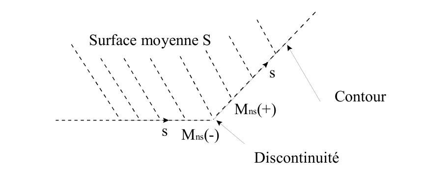
Figure 3.3.2-a: Boundary condition with angular points for a plate element

Note:

Love-Kirchhoff kinematics implies that on the contour of the plate the transverse shear force is linked to the torsional moment. It can be seen that the order of the bending equilibrium equations is higher than with Hencky kinematics. Thus, choosing Love‑Kirchhoff kinematics amounts to increasing the degree of interpolation functions because greater regularity is required for the arrow terms compared to the membrane terms due to the presence of second derivatives of the arrow in the expression of the work of the deformations. None of the Code_Aster plate elements use this kinematics. There may therefore be differences between the results obtained with the Code_Aster elements and the analytical results obtained using Love-Kirchhoff kinematics for structures with angular contours.

3.3.3. Main boundary conditions encountered [1]

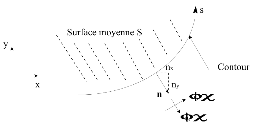
Figure 3.3.3-a: Boundary condition for a plate element

The boundary conditions frequently encountered are grouped together in the following table. They are given for the Hencky kinematics in the coordinate system defined by s and the external normal to the plate:

Embed	Simple Support	Free Edge	Symmetry with respect to an axis \(s\)	Antisymmetry with respect to an axis \(s\)
\(\begin{array}{}\stackrel{ˉ}{u}=\mathrm{0,}\\ \stackrel{ˉ}{v}=\mathrm{0,}\\ \stackrel{ˉ}{w}=\mathrm{0,}\\ {\stackrel{ˉ}{\theta }}_{s}=\mathrm{0,}\\ {\stackrel{ˉ}{\theta }}_{n}=0\text{.}\end{array}\)	\(\begin{array}{}{\stackrel{ˉ}{u}}_{n}=\mathrm{0,}\\ \stackrel{ˉ}{w}=\mathrm{0,}\\ {\stackrel{ˉ}{\theta }}_{n}=0\text{.}\end{array}\)		\(\begin{array}{}{\stackrel{ˉ}{u}}_{n}=\mathrm{0,}\\ {\stackrel{ˉ}{\theta }}_{s}=0\text{.}\end{array}\)	\(\begin{array}{}{\stackrel{ˉ}{u}}_{s}=\mathrm{0,}\\ \stackrel{ˉ}{w}=\mathrm{0,}\\ {\stackrel{ˉ}{\theta }}_{n}=0\text{.}\end{array}\)
	\(\begin{array}{}{\phi }_{s}=\mathrm{0,}\\ {\chi }_{s}=0\text{.}\end{array}\)	\(\begin{array}{}{\phi }_{s}=\mathrm{0,}\\ {\phi }_{n}=\mathrm{0,}\\ {\phi }_{z}=\mathrm{0,}\\ {\chi }_{s}=\mathrm{0,}\\ {\chi }_{n}=0\end{array}\)	\(\begin{array}{}{\phi }_{s}=\mathrm{0,}\\ {\phi }_{z}=\mathrm{0,}\\ {\chi }_{n}=0\text{.}\end{array}\)	\(\begin{array}{}{\phi }_{n}=\mathrm{0,}\\ {\chi }_{s}=0\text{.}\end{array}\)

with: \(\begin{array}{}{u}_{n}={\text{un}}_{x}+{\text{vn}}_{y};{u}_{s}\text{=-}{\text{un}}_{y}+{\text{vn}}_{x},\\ {\theta }_{n}={\theta }_{x}{n}_{x}+{\theta }_{y}{n}_{y};{\theta }_{s}=-{\theta }_{x}{n}_{y}+{\theta }_{y}{n}_{x},\\ {\phi }_{n}={\phi }_{x}{n}_{x}^{2}+2{\phi }_{\text{xy}}{n}_{x}{n}_{y}+{\phi }_{y}{n}_{y}^{2},\\ {\phi }_{s}=-{\phi }_{x}{n}_{x}{n}_{y}+{\phi }_{\text{xy}}({n}_{x}^{2}-{n}_{y}^{2})+{\phi }_{y}{n}_{x}{n}_{y},\\ {\chi }_{n}={\chi }_{x}{n}_{x}^{2}+2{\chi }_{\text{xy}}{n}_{x}{n}_{y}+{\chi }_{y}{n}_{y}^{2},\\ {\chi }_{s}=-{\chi }_{x}{n}_{x}{n}_{y}+{\chi }_{\text{xy}}({n}_{x}^{2}-{n}_{y}^{2})+{\chi }_{y}{n}_{x}{n}_{y}\text{.}\end{array}\) Note: we have \(\begin{array}{}{\beta }_{s}=-{\theta }_{n},\\ {\beta }_{n}={\theta }_{s}\text{.}\end{array}\).