2. Formulation#
2.1. Geometry of plate elements [1]#
For plate elements, a reference surface, or average, plane surface is defined (plane \(x,y\) for example) and a thickness \(h(x,y)\). This thickness must be small compared to the other dimensions (extensions, radii of curvature) of the structure to be modelled. The [Figure 2.1-a] below illustrates our point.
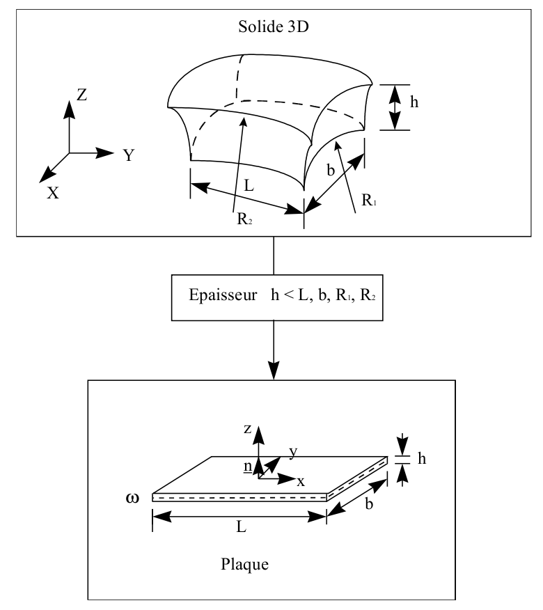
Figure 2.1-a
A local orthonormal coordinate system \(\mathit{Oxyz}\) associated with the tangential plane of the structure different from the global coordinate system \(\mathit{OXYZ}\) is attached to the mean surface \(\omega\). The position of the points on the plate is given by the Cartesian coordinates \((x,y)\) of the mean surface and the elevation \(z\) with respect to this surface.
2.1.1. Intrinsic coordinate system#
By taking the previous local coordinate system \(\mathit{Oxyz}\) with the first vertex of the element as its origin and the \(\mathit{Ox}\) axis being the side joining vertices 1 and 2, we define the so-called intrinsic coordinate system.
2.2. Plate theory#
These elements are based on the theory of plates in small displacements and small deformations.
2.2.1. Cinematics#
Straight sections that are sections perpendicular to the mean surface remain straight; material points located on a normal to the undeformed mean surface remain on a line in the deformed configuration. As a result of this approach, the displacement fields vary linearly in the plate thickness. If we designate by \(u,v,w\) the movements from a point \(q(x,y,z)\) following \(x\), \(y\) and \(z\), we thus have the Hencky-Mindlin kinematics:
where \(u,v,w\) are the movements of the mean surface and \({\theta }_{x}\) and \({\theta }_{y}\) the rotations of this surface with respect to the two axes \(x\) and \(y\) respectively. It is preferred to introduce the two \({\mathrm{\beta }}_{x}(x,y)={\mathrm{\theta }}_{y}(x,y),{\mathrm{\beta }}_{y}(x,y)=-{\mathrm{\theta }}_{x}(x,y)\) rotations.
The three-dimensional deformations at any point, with the kinematics introduced earlier, are thus given by:
where \({e}_{\text{xx}},{e}_{\text{yy}}\) and \({e}_{\text{xy}}\) are the membrane strains of the mean surface, \({\mathrm{\gamma }}_{x}\) and \({\mathrm{\gamma }}_{y}\) the deformations associated with transverse shears, and \({\mathrm{\kappa }}_{\text{xx}},{\mathrm{\kappa }}_{\text{yy}},{\mathrm{\kappa }}_{\text{xy}}\) the flexural deformations (or variations in curvature) of the mean surface, which are written as:
Note:
In plate theories the introduction of \({\beta }_{x}\) and \({\beta }_{y}\) makes it possible to symmetrize the formulations of deformations and, as we will see later, the equilibrium equations. In shell theories we instead use \({\theta }_{x}\) and \({\theta }_{y}\) and the associated couples \({M}_{x}\) and \({M}_{y}\) versus \(x\) and \(y\) .
2.2.2. Law of behavior#
The behavior of the plates is a 3D behavior under « plane stresses ». The transverse constraint \({\sigma }_{\text{zz}}\) is zero because it is considered to be negligible compared to the other components of the stress tensor (hypothesis of plane stresses). The most general law of behavior is then written as follows:
: label: eq-4
(begin {array} {c} {sigma}} _ {text {xx}}\ {sigma}}\ {sigma}}\ {sigma} _ {text {xy}}\ {sigma}}\ {sigma} _ {text {xz}} _ {text {xz}}}\ {sigma} _ {text {yz}}}\ {sigma}}\ end {array}} _ {text {xy}}}\ text {xy}}}\ {sigma} _ {text {xy}}}\ text {xy}}}\ {sigma} _ {text {xy}}}\ text {xy}}}\ {sigma} _ {text {xy}}}alpha) (begin {array} {c} {varepsilon}} _ {text {xx}}\ {varepsilon} _ {text {yy}}\ {gamma} _ {text {xy}} _ {text {xy}}}}\ {gamma} _ {\ gamma} _ {\ gamma} _ {y}end {array}} _ {y}end {array}} _ {gamma} _ {y}end {array}) =text {Ce} +ztext {C}kappa +text {C}gamma
textrm {with}
e= (begin {array} {c} {e} _ {text {x}}}\ {e}}\ {e}}\ 2 {e} _ {text {xy}}\ 0\0\ 0\ 0\ 0end {array}),kappa = (begin {array}} {array}}\ {array}),kappa = (begin {array} {c}} {kappa} _ {text {xy}}\ 0\0\ 0\ 0\ 0\ 00\ 00end {array}}),kappa = (begin {array}} {array}}\ {array}} _ {text {yy}}\ 2 {kappa} _ {text {x}}\ 0\ 0end {array})text {and}gamma = (begin {array} {c} 0\ 0\ 0\ 0\ 0\ 0\ 0\ {gamma} _ {x}{gamma} _ {y}end {array} {c} 0\ 0\ 0\ 0\ {gamma} _ {y}end {array} {c} 0\ 0\ 0\ 0\ {gamma} _ {y}end {array} {c} 0\ 0\ 0\ 0\ {gamma} _ {y}end {array} {c}
where \(\text{C}(e,\alpha )\) is the local tangent stiffness matrix combining plane stresses and transverse distortion and \(\alpha\) represents all the internal variables when the behavior is nonlinear.
For behaviors where transverse distortions are decoupled from membrane and flexural deformations, \(\text{C}(e,\alpha )\) takes the form:
: label: eq-5
text {C} = (begin {array} {cc} {cc}text {H} & 0\ 0& {text {H}}} _ {gamma}end {array})
where \(\text{H}(e,\alpha )\) is a \(3\mathrm{\times }3\) matrix and \({\text{H}}_{\gamma }(e,\alpha )\) is a \(2\mathrm{\times }2\) matrix. We will remain within the framework of this hypothesis.
For an isotropic homogeneous linear elastic behavior, we thus have:
where \(k\) is the transverse shear correction factor whose meaning is given in the next paragraph.
Note:
We do not describe the variation in thickness or that of the transverse deformation \({e}_{\text{zz}}\) which can however be calculated using the previous hypothesis of plane stresses. Moreover, there are no restrictions on the type of behavior that can be represented.
2.2.3. Taking into account transverse shear [2]#
Taking transverse shear into account depends on correction factors determined a priory by energy equivalences with 3D models, so that the transverse shear stiffness of the plate model is as close as possible to that defined by the theory of three-dimensional elasticity. Two theories including shear deformation exist and are presented in [2].
2.2.3.1. The so-called Hencky theory#
This theory, as well as that of Love-Kirchhoff, which immediately follows from it, is based on the kinematics presented in §2.2.1. The behavioral relationship is usual and the shear correction factor is \(k\mathrm{=}1\).
Note:
When transversal distortions \({\gamma }_{x}\) and \({\gamma }_{y}\) are not taken into account in Hencky’s theory, the model obtained is that of Love-Kirchhoff (finite elements DKT (G) and DKQ (G)). The two rotations of the mean surface are then linked to the movements of the average surface by the following relationship:
\(\begin{array}{c}{\mathrm{\beta }}_{x}=-\frac{\partial w}{\partial x}\\ {\beta }_{y}=-\frac{\partial w}{\partial y}\end{array}\)
2.2.3.2. The so-called Reissner theory (DST, DSQ and Q4g)#
The second theory, called Reissner’s, is developed on the basis of constraints. The variation in membrane stresses (\({\sigma }_{\mathrm{xx}}\), \({\sigma }_{\mathrm{yy}}\) and \({\mathrm{\sigma }}_{\mathit{xy}}\)) is assumed to be linear in thickness as in the case of Hencky’s theory where this results from the linearity of the variation of membrane deformations with thickness.
However, while it is assumed, in Hencky’s theory, that the distortion is constant in thickness and therefore in shear stresses, which violates boundary conditions \({\mathrm{\sigma }}_{\mathit{xz}}={\mathrm{\sigma }}_{\mathit{yz}}=0\) on the upper and lower faces of the plate due to the law of behavior set out in §2.2.2., in the context of Reissner’s theory, we use the equilibrium equations to derive/establish the variation of shear stresses. in the thickness of the plate, in particular while respecting the conditions of balance on the faces upper and lower plate. The internal energy of the model obtained after solving the equilibrium equations in 3D, for bending only, with the variation of the plane stresses according to \(z\), reveals, for an elastic material, a relationship between the resulting forces and the average rotations and the average deflection. It is in this relationship that the shear correction factor of \(k\mathrm{=}5\mathrm{/}6\) appears instead of \(1\) in the relationship that links shear force to distortion for a homogeneous and isotropic plate. The determination of shear correction factors for orthotropic plates or laminated plates is described in the appendix.
2.2.3.3. Equivalence of the Hencky-Love-Kirchhoff and Reissner approaches#
If we equate the slopes of the mean surface \({\mathrm{\beta }}_{x},{\mathrm{\beta }}_{y}\) to the averages of the slopes in the thickness of the plate and the arrow \(w\) to the mean arrow, the only difference between Hencky’s theory and that of Reissner is the transverse shear correction coefficient in homogeneous isoptropic elasticity of \(5\mathrm{/}6\) instead of \(1\). This difference is due to the fact that the initial hypotheses are of a different nature and especially that the variables chosen are not the same. In fact, the arrow on the mean surface is not equal to the average of the arrows on the thickness of the plate. It is therefore normal that behavioral relationships that involve different variables are not the same step.
The fact of having to solve displacement problems at the finite element level rather than constraint problems by interpolation of movements leads us to use the equivalent displacement approach of the Reissner problem formulated in constraints.
2.2.3.4. notes#
Because of the previous equivalence, only the moving model is presented here for all the elements. In fact the elements DKT, DKTG, DKQG and DKQ are based on the Hencky-Love-Kirchhoff theory and the elements DST, DSQ and Q4G are based on the Reissner theory.
The determination of correction factors is based on another theory, that of Mindlin, on natural frequency equivalences associated with the mode of vibration by transverse shear. We then obtain \(k={\mathrm{\pi }}^{2}/12\), a value very close to \(5\mathrm{/}6\) for the elements DST, DSQ and Q4G in the isotropic case.
In the context of plasticity, the problem of choosing the transverse shear correction coefficient arises because the equivalent displacement approach of the Reissner problem formulated in constraints involves the non-linearity of the behavior. It is therefore not possible to derive/to establish from this, as is the case for elastic materials, a value of the transverse shear correction coefficient. Plasticity (and other non-linear behaviors) is therefore not developed for these elements.
2.2.3.5. Calculating shear stress and transverse distortion in code_aster#
The calculation of the shear stress is carried out by considering:
the equilibrium equations in stress and in generalized effort:
the \({\mathrm{\sigma }}_{\mathit{xz}}(-h/2)={\mathrm{\sigma }}_{\mathit{yz}}(h/2)=0\) free edge conditions on the upper and lower sides;
relationships linking plane constraints to the derivatives of moments:
Or after analytic integration with respect to the variable \(z\) of \({\mathrm{\sigma }}_{\mathit{xz}}(z),{\mathrm{\sigma }}_{\mathit{yz}}(z)\) and identification of the coefficients of the primitive:
the expression of shear stress:
\({\mathrm{\sigma }}_{\mathit{xz}}={T}_{x}\cdot 3/2h\ast (1-4{z}^{2}/{h}^{2})\) \({\mathrm{\sigma }}_{\mathit{yz}}={T}_{y}\cdot 3/2h\cdot (1-4{z}^{2}/{h}^{2})\)
the expression of shear deformation in the framework of Reissner’s theory:
\({\mathrm{\gamma }}_{x}={\mathrm{\tau }}_{\mathit{xz}}\cdot 2(1+\mathrm{\nu })/\mathit{Ek}\) \({\gamma }_{y}={\tau }_{\mathrm{yz}}\cdot 2(1+\nu )/\mathrm{Ek}\) with \(k\) the shear correction coefficient
the expression of shear deformation in the framework of Kirchoff’s theory:
\({\gamma }_{x}={\tau }_{\mathrm{xz}}\cdot 2(1+\nu )/\mathrm{Ek}-{\partial }_{x}w\) \({\mathrm{\gamma }}_{y}={\mathrm{\tau }}_{\mathit{yz}}\cdot 2(1+\mathrm{\nu })/\mathit{Ek}-{\partial }_{y}w\)
This is an approximation that is also found in [3] (eq 9).
We generalize the expression of shear stresses by introducing a function \(d1\mathit{iel}(z)\) such as:
\({\mathrm{\sigma }}_{\mathit{xz}}={T}_{x}\cdot d1\mathit{iel}(z)\) \({\mathrm{\sigma }}_{\mathit{yz}}={T}_{y}\cdot d1\mathit{iel}(z)\)
In classic cases, we have: \(d1\mathit{iel}(z)=3/(2h)\cdot (1-4{z}^{2}/{h}^{2})\).
In more general cases (in the presence of the eccentricity for example) \(d1\mathit{iel}(z)\) must be modified to take into account the phenomenon in question. To correctly approximate the shear stress, the choice is made to apply a general quadratic form for \(d1\mathit{iel}(z)=a\cdot {z}^{2}+b\cdot z+c\) such that the following conditions are met:
\(\underset{-h/2}{\overset{h/2}{\int }}d1\mathit{iel}(z)=1\) shear effort-constraints relationship
\(d1\mathit{iel}(z=-h/2)=0;d1\mathit{iel}(z=h/2)=0\) free edge condition
The first condition makes it possible to automatically respect the equilibrium relationships in linear elasticity while the second makes it possible to find correct results on the unconstrained edges. Extending these relationships to plasticity is not trivial. However, in plasticity, it is chosen to keep a linear elastic description of shear stresses.
The expression of \(d1\mathit{iel}(z)\) in the case of eccentricity is explained in the dedicated reference doc [R3.07.06].