6. Conclusion#
The finite elements of plane plates that we describe here are used in the calculations of thin structures, in small displacements and deformations, whose characteristic thickness-to-length ratio is less than \(1\mathrm{/}10\). As these elements are flat, they do not take into account the curvature of the structures, and it is necessary to refine the meshes in case it is important.
They are elements for which the deformations and stresses in the plane of the element vary linearly with the thickness of the plate. In addition, the distortion associated with transverse shear is constant in the thickness of the element. Two families of finite plate elements exist: elements DKT, DKQ (or DKTG, DKQG) for which the transverse distortion is zero and the finite elements with transverse shear energy DST, DSQ and Q4G (or Q4G) for which it remains constant and not zero in thickness. It is recommended to use the second type of elements when the structure to be studied has a characteristic thickness-to-length ratio between \(1\mathrm{/}20\) and \(1\mathrm{/}10\) and the former in the rest of the cases. When the transverse distortion is non-zero, the plate elements DST, DSQ and Q4G do not satisfy the 3D equilibrium conditions and the boundary conditions on the nullity of the transverse shear stresses on the upper and lower faces of the plate, compatible with a constant transverse distortion in the thickness of the plate. As a result, at the level of elastic behavior, a coefficient of \(5\mathrm{/}6\) for a homogeneous plate corrects the usual relationship between the stresses and the transverse distortion in order to ensure equality between the shear energies of the 3D model and of the plate model with constant distortion. In this case, arrow \(w\) interprets the mean transverse displacement in the thickness of the plate.
Nonlinear behaviors under plane constraints are available for plate elements DKT and DKQ only. In fact, the rigorous consideration of a constant non-zero transverse shear on the thickness and the determination of the associated correction on the shear stiffness with respect to a model satisfying the equilibrium conditions and the boundary conditions are not possible and therefore make the use of elements DST, DSQ and Q4G strictly impossible in plasticity.
For the elements of the DKTG family, only global behavioral relationships (relationships between moment and curvature and membrane forces — elongations) are available.
Elements corresponding to mechanical elements exist in thermal engineering; thermomechanical linkages are therefore available except, for the moment, for laminated materials.
: Orthotropic plates
For an orthotropic material like the one shown in the figure, composed for example of fibers of direction \(L\) coated with a matrix, whose orthotropic axes are \(L\), \(T\) and \(Z\) with isotropy of axis \(L\), the expression for the matrices \(\text{H}\) and \({\text{H}}_{\mathrm{\gamma }}\) in the orthotropic coordinate system previously defined becomes:
with \(\begin{array}{c}{H}_{\text{LL}}=\frac{{E}_{L}}{1-{\mathrm{\nu }}_{\text{LT}}{\mathrm{\nu }}_{\text{TL}}};{H}_{\text{TT}}=\frac{{E}_{T}}{1-{\mathrm{\nu }}_{\text{LT}}{\mathrm{\nu }}_{\text{TL}}}\\ {H}_{\text{LT}}=\frac{{E}_{T}{\mathrm{\nu }}_{\text{LT}}}{1-{\mathrm{\nu }}_{\text{LT}}{\mathrm{\nu }}_{\text{TL}}}=\frac{{E}_{L}{\nu }_{\text{TL}}}{1-{\mathrm{\nu }}_{\text{LT}}{\mathrm{\nu }}_{\text{TL}}}\end{array}\) and \(\begin{array}{c}{G}_{\text{LZ}}=\frac{{E}_{L}}{2(1+{\mathrm{\nu }}_{\text{LZ}})}\\ {G}_{\text{TZ}}=\frac{{E}_{T}}{2(1+{\mathrm{\nu }}_{\text{TZ}})}\end{array}\).
Knowledge of the five independent coefficients \({E}_{L}\), \({E}_{T}\),, \({G}_{\text{LT}}\), \({G}_{\text{TZ}}\) and \({\nu }_{\text{LT}}\) is sufficient to determine the coefficients of the matrices \(\text{H}\) and \({\text{H}}_{\gamma }\) since:
\({\mathrm{\nu }}_{\text{TL}}=\frac{{E}_{T}{\mathrm{\nu }}_{\text{LT}}}{{E}_{L}}\) and \({G}_{\text{LZ}}={G}_{\text{LT}}\).
If we designate by \(\theta\) the angle between the orthotropy coordinate system and the main axis of the coordinate system defined by the user using ANGL_REP we establish that:
: label: eq-50
text {H} = {text {T}}} _ {1} ^ {T} {text {H}} _ {L} {text {T}}} _ {1}
textrm {and}
{text {H}} _ {mathrm {gamma}}} = {text {T}} _ {2} ^ {T} {text {H}} _ {Lmathrm {gamma}} {mathrm {gamma}}}} {text {T}} _ {2}
with: \({\text{T}}_{1}=\left(\begin{array}{ccc}{C}^{2}& {S}^{2}& \text{CS}\\ {S}^{2}& {C}^{2}& -\text{CS}\\ -2\text{CS}& 2\text{CS}& {C}^{2}-{S}^{2}\end{array}\right)\) and \({\text{T}}_{2}=\left(\begin{array}{cc}C& S\\ -S& C\end{array}\right)\) where \(C=\text{cos}\mathrm{\theta },S=\text{sin}\mathrm{\theta }\) and \(\mathrm{\theta }=(x,L)\) as shown in the figure below.
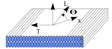
Figure 6-1: Composite plate
In the case of initial thermal stresses, we also have:
where \({\alpha }_{L}\) and \({\alpha }_{T}\) are the coefficients of thermal expansion in the directions \(L\) and \(T\) and \(\Delta T\) the temperature variation.
: Transverse shear correction factors for orthotropic or laminated plates The matrix \({\text{H}}_{\text{ct}}\) is defined so that the surface density of transverse shear energy obtained in the case of the three-dimensional distribution of stresses resulting from the resolution of the equilibrium is equal to that of the plate model based on Reissner’s hypotheses, for simple flexural behavior. We should therefore find \({\text{H}}_{\text{ct}}\) such as:
: label: eq-52
frac {1} {2}underset {-h/2} {overset {-h/2} {int}}tau {text {H}} _ {gamma} ^ {-1}tau =frac {1} {2} {2} {frac {1} {2} {2} {2} {text {TH}}} _ {text {ct}}} ^ {-1}text {T}} =frac {1} {2}gamma {text {H}}} _ {text {ct}}gamma
textrm {with}
tau = (begin {array} {c} {c} {sigma} _ {text {xz}} _ {text {yz}}end {array}) and:math:text {T} =text {T} =underset {-h/2}} {overset {-h/2} {sigma} _ {text {yz}}}end {array}) and:math:text {T}} =text {T} =underset {-h/2} {overset {-h/2} {int}}tautext {dz}} = {text {T}} = {text {T}} = {text {T}} =underset {-h/2} {text {H}} _ {text {ct}}gamma
To obtain \({\text{H}}_{\text{ct}}\) we use the distribution of \(\tau\) following \(z\) obtained from the resolution of the 3D equilibrium equations without external torques:
\({\sigma }_{\text{xz}}=-\underset{-h/2}{\overset{z}{\int }}({\sigma }_{\text{xx},x}+{\sigma }_{\text{xy},y})d\zeta ;{s}_{\text{yz}}=-\underset{-h/2}{\overset{z}{\int }}({\sigma }_{\text{xy},x}+{\sigma }_{\text{yy},y})d\zeta\) with \({\sigma }_{\text{xz}}={\sigma }_{\text{yz}}=0\) for \(z=\pm h/2\).
In the case where there is no membrane-flexure coupling (symmetry with respect to \(z\mathrm{=}0\)), the stresses in the plane of the element \({\sigma }_{\text{xx}}\), \({\sigma }_{\text{yy}}\) and \({\sigma }_{\text{xy}}\) are expressed in the case of pure flexural behavior:
\(\sigma =z\text{A}(z)\text{M}\) with \(\text{A}(z)=\text{H}(z){\text{H}}_{f}^{-1}\).
If \(\text{H}(z)\) and \({\text{H}}_{f}\) do not depend on \(x\) and \(y\) we can determine \({\text{H}}_{\text{ct}}\). In fact:
\(\tau (z)={\text{D}}_{1}(z)\text{T}+{\text{D}}_{2}(z)\lambda\) where \(\text{T}=(\begin{array}{c}{T}_{x}\\ {T}_{y}\end{array})=(\begin{array}{c}{M}_{\text{xx},x}+{M}_{\text{xy},y}\\ {M}_{\text{xy},x}+{M}_{\text{yy},y}\end{array})\) and \(\lambda =(\begin{array}{c}{M}_{\text{xx},x}-{M}_{\text{xy},y}\\ {M}_{\text{xy},x}-{M}_{\text{yy},y}\\ {M}_{\text{yy},x}\\ {M}_{\text{xx},y}\end{array})\)
as well as:
\({\text{D}}_{1}=-\underset{-h/2}{\overset{z}{\int }}\frac{\zeta }{2}(\begin{array}{cc}{A}_{\text{11}}+{A}_{\text{33}}& {A}_{\text{13}}+{A}_{\text{32}}\\ {A}_{\text{31}}+{A}_{\text{23}}& {A}_{\text{22}}+{A}_{\text{33}}\end{array})d\zeta\),
\({\text{D}}_{2}\text{=-}\underset{-h/2}{\overset{z}{\int }}\frac{\zeta }{2}(\begin{array}{cccc}{A}_{\text{11}}-{A}_{\text{33}}& {A}_{\text{13}}-{A}_{\text{32}}& 2{A}_{\text{12}}& 2{A}_{\text{31}}\\ {A}_{\text{31}}-{A}_{\text{23}}& {A}_{\text{33}}-{A}_{\text{22}}& 2{A}_{\text{32}}& 2{A}_{\text{21}}\end{array})d\zeta\).
As a result, \(\frac{1}{2}\underset{-h/2}{\overset{+h/2}{\int }}\tau {\text{H}}_{\gamma }^{-1}\tau =\frac{1}{2}(\begin{array}{c}\text{T}\\ \lambda \end{array})(\begin{array}{cc}{C}_{\text{11}}& {C}_{\text{12}}\\ {C}_{\text{12}}^{T}& {C}_{\text{22}}\end{array})(\begin{array}{c}\text{T}\\ \lambda \end{array})\) with: \(\begin{array}{c}{\text{C}}_{\text{11}}=\underset{-h/2}{\overset{+h/2}{\int }}{\text{D}}_{1}^{T}{\text{H}}_{\mathrm{\gamma }}^{-1}{\text{D}}_{1}\text{dz};\\ {\text{C}}_{\text{12}}=\underset{-h/2}{\overset{+h/2}{\int }}{\text{D}}_{1}^{T}{\text{H}}_{\mathrm{\gamma }}^{-1}{\text{D}}_{2}\text{dz};\\ {\text{C}}_{\text{22}}=\underset{-h/2}{\overset{+h/2}{\int }}{\text{D}}_{2}^{T}{\text{H}}_{\mathrm{\gamma }}^{-1}{\text{D}}_{2}\text{dz}\end{array}\)
As in addition \(\frac{1}{2}\underset{-h/2}{\overset{+h/2}{\int }}\tau {\text{H}}_{\gamma }^{-1}\tau =\frac{1}{2}{\text{TH}}_{\text{ct}}^{-1}\text{T}\), we propose to take \({\text{H}}_{\text{ct}}={\text{C}}_{\text{11}}^{-1}\) to best satisfy the two equations regardless of \(T\) and \(\lambda\).
By comparing \({\text{H}}_{\text{ct}}\) calculated in this way with \({\stackrel{ˉ}{\text{H}}}_{\text{ct}}=\underset{-h/2}{\overset{+h/2}{\int }}{\text{H}}_{\gamma }\text{dz}\), the following transverse shear correction coefficients are shown:
For a homogeneous, isotropic or anisotropic plate, we thus find: \({\text{H}}_{\text{ct}}=\mathrm{kh}{\text{H}}_{\gamma }\) with \(k\mathrm{=}5\mathrm{/}6\).
Notes:
This method is only valid when the composite plate is symmetric with respect to \(z\mathrm{=}0\) .
For a multilayer material, it is established that:
where: \({h}_{i}={z}_{i+1}-{z}_{i},{\eta }_{i}=\frac{1}{2}({z}_{i+1}+{z}_{i})\) and \({\text{A}}_{i}\) represent the \((\begin{array}{cc}{A}_{\text{11}}+{A}_{\text{33}}& {A}_{\text{13}}+{A}_{\text{32}}\\ {A}_{\text{31}}+{A}_{\text{23}}& {A}_{\text{22}}+{A}_{\text{33}}\end{array})\) matrix for layer \(i\).
The validity of choice \({\text{H}}_{\text{ct}}={\text{C}}_{\text{11}}^{-1}\) can be examined a posteriori when we have an estimate of the solution (fields of displacement and plane constraints, in particular). We can then estimate the difference between the two energy estimates. A two-step calculation approach for multilayer plates and shells (with \({\text{H}}_{\text{ct}}\) diagonal and two coefficients \({k}_{1}\) and \({k}_{2}\)) has also been developed by Noor and Burton [8] and [8].
In the case of an isotropic or anisotropic homogeneous plate, the equality between the two energies is satisfied in the strict sense since \({\text{D}}_{2}=0\). The choice made above is then valid and no subsequent examination is necessary.