2. Description of the method#
2.1. The case of linear elasticity#
In this section, we will present Hybrid High-Order (HHO) methods using the linear elasticity problem. The aim is to describe the main principles of constructing methods HHO. For simplicity, we assume that domain \(\Omega_{0}\subset \mathbb{R}^{d}\), with \(2\le d\le 3\), is a polyhedral domain that is bounded, connected and with a Lipschitzian border \(\Gamma =\partial \Omega_{0}\). Domain \(\Omega_{0}\) is deformed under the action of volume loading \(f \in {L}^{2}(\Omega_0;\mathbb{R}^{d})\) and homogeneous Dirichlet conditions are imposed on edge \(\Gamma\) (for simplicity). The weak formulation of the problem is:
Where \({H}_{0}^{1}(\Omega_0;\mathbb{R}^{d})=\{v \in {H}^{1}(\Omega_0;\mathbb{R}^{d}) : v=0 \text{ sur } \Gamma \}\) and \(\mu>0\) and \(\lambda\ge 0\) are the Lamé parameters of the material. Additionally, \(\nabla^{s}\) refers to the symmetric part of the gradient operator and \(\nabla \cdot\) the divergence operator.
2.2. Discreet frame#
2.2.1. Meshing#
We consider a \({(\mathcal{T}_{h})}_{h>0}\) mesh family, where for each \(h>0\), mesh \(\mathcal{T}_{h}\) is composed of open, disjunct, non-empty polyhedra, which have flat faces, and such as \({\overline\Omega}_{0}={\cup }_{T \in \mathcal{T}_{h}}\overline{T}\). The overall size of the mesh is described by the parameter \(h=\max_{T \in \mathcal{T}_{h}}{h}_{T}\), where \({h}_{T}\) is the diameter of cell \(T\). A closed subset \(F\) of \({\overline\Omega}_{0}\) is called a face if it is a subset having a non-empty relative interior contained in an affine hyperplane \({H}_{F}\) and if:
or there are two distinct \({T}_{1},{T}_{2} \in \mathcal{T}_{h}\) cells such as \(F=\partial {T}_{1}\cap \partial {T}_{2}\cap {H}_{F}\) (and \(F\) is then called an interface)
or there is a \(T \in \mathcal{T}_{h}\) cell such as \(F=\partial T\cap \Gamma \cap {H}_{F}\) (and \(F\) is then called an edge face).
The faces of the mesh are combined within the set \(\mathcal{F}_{h}\), which is thus partitioned. into two subsets, \(\mathcal{F}_{h}^{i}\) the set of interfaces and \(\mathcal{F}_{h}^{b}\) the set of edge faces. For all \(T \in \mathcal{T}_{h}\), \({F}_{T}\) refers to the set of mesh faces that are included in \(\partial T\) and \({n}_{T}\) the unitary outgoing normal to cell \(T\). In the following, we assume that the \({(\mathcal{T}_{h})}_{h>0}\) mesh family is regular in the sense specified in [3], i.e. for all \(h>0\), there is a conformal sub-mesh of \(\mathcal{T}_{h}\) composed of simplexes Which belongs to a regular family of simplicial meshes in the usual Ciarlet sense and such that each cell \(T \in \mathcal{T}_{h}\) of the mesh (respectively, each face \(F \in \mathcal{F}_{h}\)) can be broken down into a uniformly bounded number of sub-cells (respectively, sub-faces) that belong only one cell in the mesh (respectively, only one face or inside a cell) with a uniformly comparable diameter.
2.2.2. Approximation#
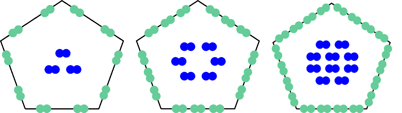
Let \(k\ge 1\) be a fixed polynomial degree. In each cell \(T \in \mathcal{T}_{h}\) of the mesh, the local HHO unknowns are the \(({v}_{T},{v}_{\partial T})\) pair, where the cell unknown \({v}_{T} \in \mathbb{P}_{d}^{k}(T;\mathbb{R}^{d})\) is a polynomial with vector values with \(d\) -degree variables at most \(k\) in cell \(T\), and \({v}_{\partial T} \in \mathbb{P}_{d-1}^{k}({F}_{T};\mathbb{R}^{d}) := {\prod }_{F \in {F}_{T}}\mathbb{P}_{d-1}^{k}(F;\mathbb{R}^{d})\) Is a polynomial with vector values defined piecewise with \((d-1)\) -degree variables at most \(k\) on each side \(F \in {F}_{T}\) of cell \(T\). In the following, we write more concisely that:
The degrees of freedom are illustrated in this représentation, where a point represents a degree of freedom (but not necessarily a physical evaluation point) and the geometric shape of the cell is illustrative only. Degrees of freedom do not make physical sense a prima facie and from an algebraic point of view, they simply correspond to the coefficients in a polynomial base.
Space \({U}_{T}^{k}\) is equipped with the following local discrete semi-standard:
with the piecewise constant function \({\gamma }_{\partial T\mid F}\) such that:
: label: eq-4
{gamma} _ {partial Tmid F} = {h} _ {F} ^ {-1},:forall Fin {F} _ {T}
where \({h}_{F}\) is the diameter of \(F\). We are also introducing the \(\mathrm{RM}(T)\) space rigid body movements on \(T\) such as:
: label: eq-5
textrm {RM} (T) :={v: Ttomathbb {R} ^ {d},mid, v (x) =c+omega x,text {where} cinmathbb {R} {R} {R}} ^ {R}} ^ {R} ^ {R}} ^ {R}} ^ {d}} ^ {d}}
where \({\mathrm{SO}}^{d}\) is the set of rotation matrices in real Euclidean space. Note that \(\nabla^{s}=0\) is equivalent to \(v \in \mathrm{RM}(T)\) and that \(\mathbb{P}_{d}^{0}(T;\mathbb{R}^{d})\subset \mathrm{RM}(T)\subset \mathbb{P}_{d}^{1}(T;\mathbb{R}^{d})\).
Lemma 1
For all \({\widehat{v}}_{T} \in {U}_{T}^{k}\), we have \(\vert{\widehat{v}}_{T}\vert{}_{1,T}=0\) If and only if \({v}_{T}\) is a rigid body movement and that \({v}_{\partial T}\) is the trace of \({v}_{T}\) on \(\partial T\).
Proof:
Note that \(\vert {\widehat{v}}_{T} \vert {}_{1,T}=0\) is equivalent to:
We deduce that \({v}_{T}\) is a rigid body movement Because \(\nabla^{s}{v}_{T}=0\) and \({v}_{\partial T}\) are the traces of \({v}_{T}\) on \(\partial T\) because \({v}_{T}-{v}_{\partial T}=0.\) ■
2.3. Local reconstruction and stabilization operators#
Methods HHO are based on the reconstruction of different discrete quantities that will come to play the role of their continuous counterpart in the formulation of the discrete problem. In the case of discretizing the linear elasticity problem, the first key ingredient is the symmetric gradient reconstruction operator \({E}_{T} : {U}_{T}^{k}\to \mathbb{P}_{d}^{k}(T;\mathbb{R}_{\mathrm{sym}}^{d\times d})\) From unknown cell \(v_T \in \mathbb{P}_{d}^{k}(T;\mathbb{R}^{d})\) and unknowns of the face \({v}_{\partial T} \in \mathbb{P}_{d-1}^{k}({F}_{T};\mathbb{R}^{d})\) component The \({\widehat{v}}_{T}=({v}_{T},{v}_{\partial T})\) pair. For everything \({\widehat{v}}_{T} \in {U}_{T}^{k}\), the reconstructed symmetric gradient \({E}_{T}({\widehat{v}}_{T}) \in \mathbb{P}_{d}^{k}(T;\mathbb{R}_{\mathrm{sym}}^{d\times d})\) is achieved by solving the following local problem: for all \(\tau \in \mathbb{P}_{d}^{k}(T;\mathbb{R}_{\mathrm{sym}}^{d\times d})\):
Solving this problem involves choosing a polynomial base of \(\mathbb{P}_{d}^{k}(T;\mathbb{R})\) only and to invert the associated mass matrix for each component of the \({E}_{T}({\widehat{v}}_{T})\) tensor.
The second key ingredient to build HHO methods is the local stabilization operator which makes it possible to weakly impose equality between the unknowns of the face \({v}_{\partial T}\) and the trace of the unknown cell \({v}_{T}\) through a penalty in the sense of least squares of the \({v}_{\partial T}-{v}_{T} \in \mathbb{P}_{d-1}^{k}({F}_{T};\mathbb{R}^{d})\) difference. The stabilization operator \({S}_{\partial T} \in \mathbb{P}_{d-1}^{k}({F}_{T};\mathbb{R}^{d})\) is defined such that, for all \({\widehat{v}}_{T}=({v}_{T},{v}_{\partial T})\):
where \({\Pi}_{\partial T}^{k}\) and \({\Pi}_{T}^{k}\) are the spotlights \(L^2\) -orthogonal on \(\mathbb{P}_{d-1}^{k}({F}_{T};\mathbb{R}^{d})\) and \(\mathbb{P}_{d}^{k}(T;\mathbb{R}^{d})\) respectively. In addition, the local operator for reconstructing a higher-order displacement field \({R}_{T} : {U}_{T}^{k}\to \mathbb{P}_{d}^{k+1}(T;\mathbb{R}^{d})\) is defined as, for everything \({\widehat{v}}_{T} \in {U}_{T}^{k}\), \({R}_{T}({\widehat{v}}_{T}) \in \mathbb{P}_{d}^{k+1}(T;\mathbb{R}^{d})\) is obtained by solving the following Neumann problem: for all \(w \in \mathbb{P}_{d}^{k+1}(T;\mathbb{R}^{d})\):
This reconstruction is uniquely defined by imposing the average value:
Like \({E}_{T}({\widehat{v}}_{T})\) is not stable in the sense that \({E}_{T}({\widehat{v}}_{T})=0\) does not necessarily mean that \({v}_{\partial T}={v}_{T}=\mathrm{cst}\), it is necessary to couple the operator \({E}_{T}\) to the stabilization operator \({S}_{\partial T}\). Thus, the addition of this stabilization term makes it possible to find a local stability property. which is needed to demonstrate the coercivity of the discrete problem.
Lemma 2 (Stability and bounded character)
Consider the symmetric gradient reconstruction operator defined by (2.4)
and the stabilization operator defined by (2.5). Let \({\gamma }_{\partial T}\) be defined by eq-4.
So, there is \(0<{\alpha}_{s}<{\alpha}_{b}<+\mathrm{ \infty }\), independent of \(h\),
such as, for all \(T \in \mathcal{T}_{h}\) and all \({\widehat{v}}_{T} \in {U}_{T}^{k}\):
Proof:
See Lemma 4 in [3] . ■
Another important property of the reconstructed symmetric gradient is a commutative property that is essential to prove the robustness of the method within the incompressible limit.
Lemma 3 (Commutativity)
For all \(T \in \mathcal{T}_{h}\) and all \(v \in {H}^{1}(T;\mathbb{R}^{d})\), the following equality is true:
where \({\widehat{I}}_{T}^{k} : {H}^{1}(T;\mathbb{R}^{d})\to {U}_{T}^{k}\) is the local discount operator such as:
Proof:
See Proposal 3 in [3] . ■
In the following, we also define the discrete divergence operator \({D}_{T} : {U}_{T}^{k}\to \mathbb{P}_{d}^{k}(T;\mathbb{R} )\) such as:
Note (Variants of methods HHO):
There are several variants of the HHO method shown here. Once the polynomial degree \(k\) fixed for face unknowns, the cell unknown can be of polynomial degree \(l \in \{k-1,k,k+1\},\:l\ge 1\) , with no change in approximation and stability properties (cf. [7] ) .
2.4. Discreet global problem HHO#
Now let’s define the discrete global problem. Let’s say:
The global unknown space HHO is defined as:
For a generic \({\widehat{v}}_{h} \in {U}_{h}^{k}\) element, we use the notation \({\widehat{v}}_{h} := ({v}_{\mathcal{T}_{h}},{v}_{\mathcal{F}_{h}})\). For any \(T \in \mathcal{T}_{h}\) cell in the mesh, we write \({\widehat{v}}_{T} \in {U}_{T}^{k}\) the local components of \({\widehat{v}}_{h}\) linked to the \(T\) cell and to the faces making up its edge \(\partial T\), and for any face \(F \in \mathcal{F}_{h}\), We note \({v}_{F}\) the component of \({\widehat{v}}_{h}\) linked to the side \(F\). Homogeneous Dirichlet boundary conditions are strongly applied to the unknowns related to edge faces. \(F \in \mathcal{F}_{h}^{b}\). To do this, we introduce the subspace:
We define function \({\Vert \cdot\Vert }_{{U}_{h,0}^{k}}\) as:
Proposal 1
The \({\Vert \cdot\Vert }_{{U}_{h,0}^{k}}\) function sets a standard on \({U}_{h,0}^{k}\).
Proof:
You just have to show that for everything \({\widehat{v}}_{h} \in {U}_{h,0}^{k}\), \({\Vert {\widehat{v}}_{h}\Vert }_{{U}_{h,0}^{k}}^{2}=0\) involves \({v}_{T}=0\) for all \(T \in \mathcal{T}_{h}\) and \({v}_{F}=0\) for all \(F \in \mathcal{F}_{h}\). Note that \({\Vert {\widehat{v}}_{h}\Vert }_{{U}_{h,0}^{k}}^{2}=0\) implies that for all \(T \in \mathcal{T}_{h}\):
Let’s take a cell \(T \in \mathcal{T}_{h}\) that has at least one edge face \(F \in {F}_{T}\cap \mathcal{F}_{h}^{b}\), so that \({v}_{F}=0\). So \({v}_{T}{\mid }_{F}=0\) because \({v}_{T}{\mid }_{F}-{v}_{F}=0\). Combining this with \(\nabla^{s}{v}_{T}=0\) and with a Korn inequality, we get \({v}_{T}=0\). Also, like \({v}_{T}{\mid }_{F\text{'}}-{v}_{F\text{'}}=0, \:\: \forall F\text{'} \in {F}_{T}\setminus F\), we deduct \({v}_{F\text{'}}=0\) for all \(F\text{'} \in {F}_{T}\). You just have to extend this reasoning layer by layer of cells until you have gone through all the cells. \(T \in \mathcal{T}_{h}\) and all sides \(F \in \mathcal{F}_{h}\). ■
The unobtrusive problem is this:
with
: label: eq-21
{a} _ {T} ({widehat {u}}} _ {T}, {widehat {v}} _ {T}) =2muleft{{({E} _ {T}} ({widehat {u}}} _ {T}), {widehat {u}}} _ {T}) ({widehat {v}} _ {T}))} _ {T}))} _ {T}) {L} ^ {2} (T)} + {({S}} _ {partial T} ({widehat {u}} _ {T}), {S} _ {partial T} ({widehat {v}}} _ {T}))} _ {{L}} _ {T}))} _ {{L} ^ {2} (partial T)}right}} +lambda {({D}} _ {T}))} _ {widehat {v}}} _ {V}} _ {T})} _ {widehat {v}}} _ {V}} _ {T}) T} ({widehat {u}} _ {T}), {D} _ {T}), {widehat {v}} _ {T}))} _ {{L} ^ {2} (T)}
The right-hand side in eq-21 is obtained by replacing continuous operators with their discrete versions
and by adding the term stabilization. We can show that there is only one solution
\({\widehat{u}}_{h} \in {U}_{h,0}^{k}\) to the problem (this stems from the local stability property of Lemma 2).
Also, since the contributions in (2.16) are calculated locally to cells, it is very easy to parallelize these calculations.
HHO methods have optimal convergence rates on general meshes both in the energy norm and in the \(L^2\) norm (with the assumption of elliptical regularity).
Theorem 1 (Error in energy norm)
Either \(k \geq 1\) and either \(u \in {H}_{0}^{1}(\Omega_0;\mathbb{R}^{d})\), the only solution to the (2.1) and \({\widehat{u}}_{h} \in {U}_{h,0}^{k}\) problem the only solution to problem (2.16). Assuming also the additional regularity \(u \in {H}^{k+2}(\Omega_0;\mathbb{R}^{d})\), there is a constant \(C>0\), independent of \(h\), \(\mu\), and \(\lambda\), such as:
Proof:
See Theorem 8 in [3] . ■
Theorem 2 (Standard error \(L^2\))
Under the hypotheses of Theorem 1 and also assuming elliptical regularity, there is a constant \(C>0\), independent of \(h\), \(\mu\), and \(\lambda\), such that:
Proof:
See Theorem 11 in [3] . ■
Theorem 1 and Theorem 2 estimates are robust to an incompressible limit. since they only involve the regularity of \(\nabla \cdot u\) according to \(\lambda\). These convergence rates are confirmed numerically as well as the robustness. Finally, it is important to remember that these convergence rates are one order higher than those obtained for finite elements. \({H}^{1}\) -conforms using polynomials of degree \(k\) in the cells.