1. Reference problem#
1.1. Geometry#
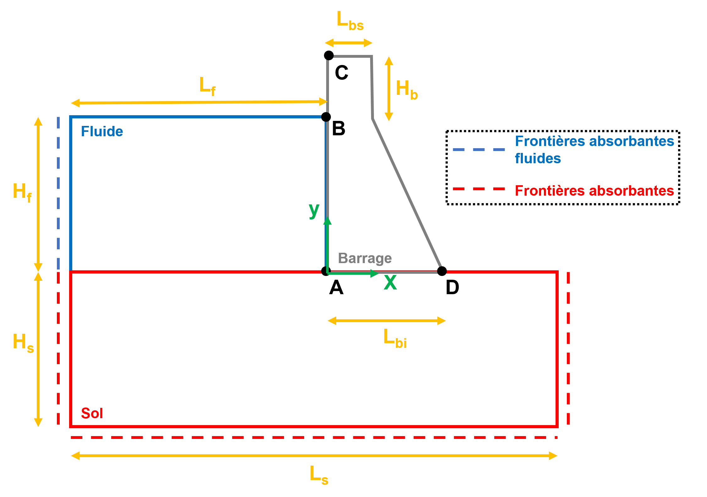
Figure 1.1-a : Geometry of the dam **** (not to scale) ** We consider a 2D dam with a geometry presented in.
In the one presented the geometric dimensions of the dam, as well as in the one specified the coordinates of the post-treatment points.
Table 1.1-1 :: Geometric dimensions of the dam**
H s |
H f |
H f |
H b |
L s |
L f |
L bi |
L bi |
L bs |
|
Measure [m] |
50 |
80 |
80 |
20 |
20 |
290 |
100 |
90 |
10 |
Table 1.1-2 : Coordinates of post-processing points
A |
B |
C |
D |
||
Coordinate X [m] |
0 |
0 |
0 |
90 |
|
Coordinate Y [m] |
0 |
0 |
80 |
100 |
0 |
1.2. Material properties#
Material properties are summarized in the.
Table 1.2-1 : Properties**of materials
E [GPa] |
\(\nu\) |
|
\(\alpha\) |
|
c e [m/s] |
||
Concrete |
22.41 |
0.2 |
0.2 |
2483 |
0.0005 |
0.75 |
|
Sol |
22.41 |
0.2 |
0.2 |
2483 |
|||
Water |
1000 |
1440 |
Where:
E is Young’s modulus;
\(\nu\) is Poisson’s ratio;
\(\rho\) is the volume density;
\(\alpha\) and \(\beta\) are the coefficients that define Rayleigh damping;
this is the speed of waves in water.
1.3. Boundary conditions and loads#
There are two types of boundary conditions (see):
At the lateral edges of the ground absorbent borders are assigned;
A fluid absorbent border is assigned to the left edge of the fluid part.
There are also two fluid-structure interfaces defined between the ground and the fluid part as well as between the dam and the fluid part. In addition, for 3D models (C and E), a periodicity condition is added in the direction in which the plane deformation is imposed.
The imposed dynamic load is a Ricker wavelet that is shown in. Charging is required for a total time of 1s. This wavelet has a direction of propagation inclined by 20° with respect to the vertical. This wavelet is injected as both a P wave and an S wave.
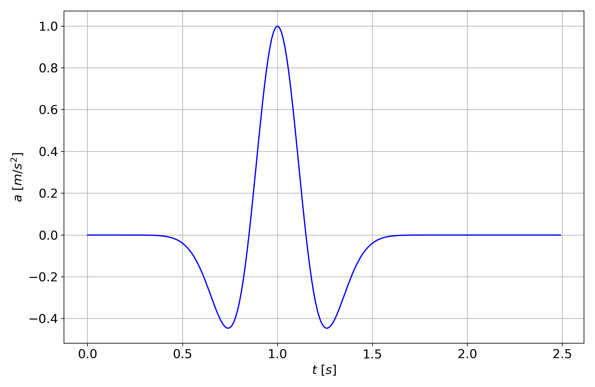
Figure 1.3-a : Ricker wavelet