1. Reference problem#
1.1. Geometry#
Miss3D uses the frequency coupling method to take into account the soil-fluid-structure interaction. This method, based on dynamic substructuring, consists in dividing the field of study into three sub-areas:
the ground,
the fluid,
the structure.
This results in 4 possible interface types:
the soil-structure interface,
the fluid-structure interface,
the free-floor interface.
Soil, fluid, and structure
The floor and the structure are made of the same homogeneous material.
In the coupled calculation*Code_Aster* - MISS3D, to represent the case of a hollow sphere of finite dimensions filled with fluid, one half of the solid medium is modelled as a « structure » domain, taken into account with*Code_Aster*, and the other half as a « ground » domain taken into account with MISS3D.
The fluid medium, which is inside the sphere with radius \(r=5m\), is taken into account with MISS3D. The solid medium occupies the volume between the spheres with radii \({r}_{\mathrm{interne}}=5m\) and \({r}_{\mathrm{externe}}=7m\).
The « structure » domain occupies the volume of solid delimited above by the equatorial horizontal plane passing through the origin of the sphere and the « ground » domain the remaining volume of solid (see Figure 1.1-a below).
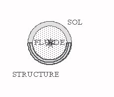
Figure 1.1-a: Domain of the ball of finite dimensions filled with fluid
Interface elements are surface elements QUAD4. The « structure » domain (in yellow in Figure 1-1.b) is modelled with volume elements HEXA8. The thickness in the radial direction is divided into four layers for a total of 1024 elements.
The maximum size of the elements is \(1.37m\), which, with a secondary wave speed in the solid of \(334m/\mathrm{sec}\), must respect the frequency limit of \(30\mathrm{Hz}\) according to the criteria:
\({l}_{\text{elem\_max}}\le \frac{{l}_{\text{onde\_max}}}{8}\) \(f\le {f}_{\mathrm{max}}=\frac{{c}_{s}}{8{l}_{\text{elem\_max}}}\)
The interfaces
In FIG. 1-1.b, the elements of the 4 interfaces are represented. Here there is a domain of free ground surface. The ground - structure interface, in black, is discretized into 128 meshes and now includes only the crown of the horizontal plane \(z=0\) between the rays \(5m\) and \(7m\). The soil-fluid interface, in dark pink, and the fluid-structure interface, in blue, are discretized in 256 meshes. The free surface in green includes the entire outer envelope of the upper hemisphere, which is also 256 meshes.
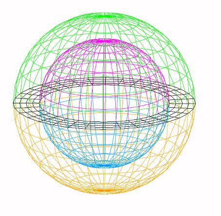
Figure 1.1-b: Surface models and meshes of interfaces
1.2. Material properties#
The ground and the structure
The mechanical characteristics of the soil and of the structure used are those indicated in table 1.1-a.
E |
\(700\mathrm{MPa}\) |
NUDE |
\(0.2\) |
RHO |
|
BETA |
|
Table 1.2-a: soil and structure characteristics
These characteristics induce a shear wave speed: \({c}_{s}=341.56m/s\) as well as a compression wave speed: \({c}_{p}=557.77m/s\)
The fluid
Celerity |
\(150m/s\) |
RHO |
|
BETA |
|
Table 1.2-b: characteristics of the fluid
A fluid velocity characteristic that is lower than the velocities of the compression shear waves is introduced into the structure and the ground in order to obtain resonances in the range of frequencies studied.
1.3. Boundary conditions and mechanical loads#
A point fluid source condition is applied to the center of the coordinate ball \((000)\) with a harmonic loading \(P={P}_{o}\mathrm{sin}\omega t\) whose pressure module \({p}_{o}\) is unitary with a pulsation that varies from \(1\mathrm{Hz}\) to \(30\mathrm{Hz}\) in steps of \(1\mathrm{Hz}\). This corresponds to a Dirac at the initial moment in time. In Code_Aster, this is the same as entering the source coordinates in CALC_MISS under the SOURCE_FLUIDE keyword.
In order not to have a rigid body movement problem, we blocked the nodes of the mesh of the structure, which are located on the axes \(X\), \(Y\) and \(Z\) respectively according to (\(Y\) and \(Z\)), (\(X\) and \(Z\)), (and), (and), (\(X\) and), (and \(Y\)), we blocked the nodes of the structure’s mesh, which are located on the axes, and respectively. Thus, the movements of rigid bodies are prevented, while allowing radial displacement.
With regard to soil-structure interface modes, it has been noted that static constraint-type modes calculated with this embedment limit condition at the soil-structure interface cannot be a complete basis for representing a spherically symmetric deformation.
To do this, new static modes have been introduced into the modal base. The modes introduced are modes of the constrained type on the external envelope of the lower hemisphere (in yellow in FIG. 1,1-b). They correspond to a new blocking limit condition according to the 3 degrees of freedom of all the nodes of this surface, except for its nodes of intersection with the axes. For these nodes, we do not have the unit mode corresponding to the degree of freedom that is tangential to the surface, because the displacement we are looking for does not have a component in this direction.
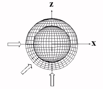


Figure 1.3-a: Radial displacement measurement points.
The best result is obtained by using a Ritz modal base without dynamic modes, and with static modes completed as indicated above. In fact, we thus have exactly the number of displacement unknowns to be determined in order to represent a spherically symmetric displacement, in particular on the structure-fluid interface.