2. Analytical solution#
2.1. Calculation method#
The monophasic unsteady and one-dimensional problem can be written in a general form such as:
\(N\frac{\partial P}{\partial t}-{K}_{i}\Delta P=0\)
\(P(t=0)={P}_{0}\)
\(P(t,x=0)=0\)
\(\frac{\partial P}{\partial x}(t,x,L)=0\)
This problem admits an analytical solution obtained by development in Fourier series.
\(P={\sum }_{k=0}^{K}\frac{{\mathrm{4P}}_{0}}{(\mathrm{2k}+1)\pi }\mathrm{exp}(\frac{-{K}_{i}}{N}{\omega }_{k}^{2}t)\mathrm{sin}({\omega }_{k}x)\) with \({\omega }_{k}=(k+\frac{1}{2})\frac{\pi }{L}\)
The number of terms \(K\) in this series is determined as follows:
Let \({n}_{x}\) be the number of \({x}_{i}\) points where the solution is evaluated at an instant \(t\).
We ask:
\({a}_{k}^{i}=\frac{4}{(\mathrm{2k}+1)\pi }\mathrm{exp}(\frac{-{K}_{i}}{N}{\omega }_{k}^{2}t)\mathrm{sin}({\omega }_{k}{x}_{i})\)
So the solution can be written as: \(P({x}_{i})={\sum }_{k=0}^{K}{P}_{0}\mathrm{.}{a}_{k}^{i}\)
We choose \(K\) such as: \(\frac{1}{{n}_{x}}\sqrt{{\sum }_{i=1}^{\mathrm{nx}}{({a}_{k}^{i})}^{2}}<\epsilon\)
In practice we took \(\varepsilon ={10}^{-10}\).
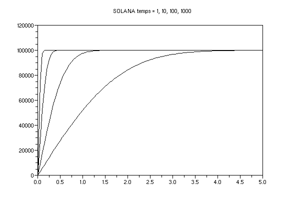
The shapes of the analytical solution at times 1, 10, 100, 1000 are shown in the figure below:
The following table shows the number of terms by time:
Time |
Number of serial terms |
1 |
194 |
10 |
64 |
100 |
22 |
1000 |
8 |
Table 2.1-1: Representation of term number as a function of time
2.2. Simplifying hypotheses#
It is considered that the medium is completely saturated with gas and a zero liquid pressure is imposed on all nodes in aster. An initial gas pressure \({P}_{g}^{\mathit{ref}}\) is imposed and boundary conditions are given which correspond to a variation in this reference pressure, so \(\delta {P}_{g}\) this pressure variation is given. The gas mass conservation equation will be written as:
\(\frac{\partial (\varphi \delta {P}_{g})}{\partial t}+d(\frac{{K}_{i}{k}_{g}}{{\mu }_{g}}({P}_{g}^{r}+\delta {P}_{g})d({P}_{g}^{r}+\delta {P}_{g}))=0\)
Assuming \(\delta {P}_{g}\) small in front of \({P}_{g}^{\mathit{ref}}\), this equation becomes:
\(\frac{\partial (\varphi \delta {P}_{g})}{\partial t}+\frac{{K}_{i}{k}_{g}}{{\mu }_{g}}{P}_{g}^{r}\Delta (\delta {P}_{g})=0\)
It is therefore \(\delta {P}_{g}\) that we will identify with the solution of the model analytical equation.
In order to find the coefficients of the model problem, we will take:
\(\varphi \mathrm{=}1\)
\({k}_{g}\mathrm{=}{\mu }_{g}\mathrm{=}1\)
and we will make sure that
\({K}_{\mathit{int}}{P}_{\mathit{ref}}\mathrm{=}{10}^{\mathrm{-}3}\).