1. Reference problem#

1.1. Geometry#

We place ourselves in the framework of 2D modeling with the hypothesis of plane deformations.

The geometry considered corresponds to a rectangular sample of 20x5 cm (the Y dimension does not matter because of the one-dimensional nature of the problem).

Point coordinates (\(m\)):

A (0; 0.05)

B (0.2; 0.05)

C (0.2; 0)

D (0; 0)

1.2. Material properties#

1.3. Only the properties on which the solution depends are given here, knowing that the command file contains other material data that ultimately does not play a role in the solution of the problem. The modeling is purely thermo-hydraulic (there is no role for mechanics).#

1.4. The sorption isotherms are explained after this table as is the relative permeability to the liquid.#

Initial reference state	Porosity Temperature T0 (\(K\)) Vapor pressure (\(\mathit{Pa}\))	0.15 293. 1000
Liquid water	Density (\({\mathrm{kg.m}}^{-3}\)) Viscosity (\({\mathrm{kg.m}}^{-1}\mathrm{.}{s}^{-1}\)) Compressibility (\({\mathrm{Pa}}^{-1}\)) Specific heat (\(J\mathrm{.}{K}^{-1}\))	1000 10-3 0.5 10-9 4180
Gas	Density (\({\mathrm{kg.m}}^{-3}\)) Viscosity (\({\mathrm{kg.m}}^{-1}\mathrm{.}{s}^{-1}\)) Specific heat (\(J\mathrm{.}{K}^{-1}\))	2 10-3 910-6 1017
Dissolved gas	Henry’s coefficient (\(\mathrm{Pa.}{\mathrm{mol}}^{-1}{m}^{3}\))	130719
Steam	Density (\({\mathrm{kg.m}}^{-3}\)) Specific heat (\(J\mathrm{.}{K}^{-1}\))	18 10-3 1900
Homogenized coefficients	Homogenized density (\({\mathit{kg.m}}^{\mathrm{-}3}\)) Intrinsic permeability \(({m}^{2})\) Relative gas permeability Thermal conductivity (\(W\mathrm{.}{K}^{-1.}{m}^{-1}\)) Specific heat (\(J\mathrm{.}{K}^{-1}\)) Diffusion in liquid mixture \(({m}^{2}\mathrm{.}{s}^{-1})\) Diffusion in the gas mixture \(({m}^{2}\mathrm{.}{s}^{-1})\)	1737 \({K}_{\text{int}}=1.2{10}^{-20}\) 1 \({\mathrm{\lambda }}_{\text{T}}=0.09S+1.34\) 1500 \({D}_{l}(S)=S\ast {10}^{-10}\) \({D}_{g}(S,T)\) (see below)

The sorption curve relating capillary pressure to saturation is given by the following relationship:

\(\mathit{Pc}(S,T)=\frac{-{\mathrm{\rho }}_{l}({T}_{0})\mathrm{.}R\mathrm{.}{T}_{0}}{\mathrm{\alpha }{M}_{\mathit{vap}}}{({S}^{-1/\mathrm{\beta }}-1)}^{1-\mathrm{\beta }}\frac{{\mathrm{\gamma }}_{\mathit{lv}}({T}_{0})}{{\mathrm{\gamma }}_{\mathit{lv}}(T)}\mathrm{.}\sqrt{\frac{m({T}_{0})}{m(T)}}\)

where \({T}_{0}\) is the reference temperature (20° C.) where the parameters \(\mathrm{\alpha }\) and \(\mathrm{\beta }\) are evaluated, R is the ideal gas constant, \({M}_{\mathit{vap}}\) is the molar mass of steam, and:

\(\frac{m(T)}{m({T}_{0})}={10}^{{A}_{d}[{2.10}^{-3}(T-{T}_{0})-{10}^{-6}{(T-{T}_{0})}^{2}]}\) and \({\mathrm{\gamma }}_{\mathit{lv}}(T)=0.1558{(1-\frac{T}{647.1})}^{1.26}\)

Moreover, the relative permeabilities are given by a Van-Genuchten relationship, such as:

\({k}_{\mathit{rl}}(S)={S}^{p}{[1-{(1-{S}^{1/\mathrm{\beta }})}^{\mathrm{\beta }}]}^{2}\)

and

\({k}_{\mathit{rg}}(S)={(1-S)}^{p}{[1-{S}^{1/\mathrm{\beta }}]}^{2.\mathrm{\beta }}\)

The constants used are [3]: \(p=2.91\) \(\mathrm{\beta }=0.389\), \(\mathrm{\alpha }=9.334\) and \({A}_{d}=10.378\)

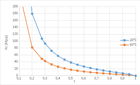
Figure 1: S (Pc) at 20°C and 60°C

Finally, the diffusion in the gas mixture [3] is such that \({D}_{g}(S,T)={D}_{0}(T){\mathrm{\varphi }}^{a}{(1-S)}^{b}\) with a and b the Milington coefficients such as a = 2.607 and b = 7 and \({D}_{0}(T)=0.217\mathrm{.}{10}^{-4}{(\frac{T}{273})}^{1.88}\).

1.5. Boundary conditions and loads#

On the left edge of the sample (edge AD), a capillary pressure is applied which corresponds to a fixed relative humidity (using Kelvin’s law) as well as a temperature:

HR = 70% (Pc = 48.2 MPa)
T = 60°C
Pg = 0.5 MPa (or 0.4 MPa compared to the initial state)
Zero flow is applied everywhere else

1.6. Initial conditions#

Initially, we uniformly consider a saturation S = 0.98, which corresponds to \({P}_{c}(x)={P}_{c0}=2.4{10}^{6}\mathit{Pa}\), a gas pressure \({P}_{g}(x)={P}_{g0}={10}^{5}\mathit{Pa}\)

and a temperature \(T(x)={T}_{0}=20°C\).