5. Summary of the results of the A, B and C models

By interpreting the diagram: math: (P, Q), with:math: P=- (2sigma’_ {xx} +sigma’_ {zz}) /3 and:math: Q=|sigma’_ {xx} -sigma’_ {zz} | for the three models A, B and C of this test case, it is clear that in modeling A, the charge remains hydrostatic up to an effective pressure value equal to \(600\) kPa. Once vertical displacement is imposed and varies over time, the pressures on the lateral faces being maintained constant, a stress diverter is induced and increases over time with positive work hardening. When we get closer to point \(Q=MP\), we tend towards perfect plasticity with plastic flow without work hardening and without any variation in constraints (see [r7.01.14]).

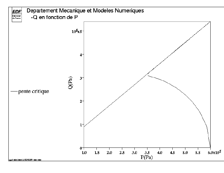
Fig. 5.1 \(Q\) based on \(P\) (modeling A).

In modeling B, after a hydrostatic loading that reaches the critical pressure at \(300\) kPa, the second charge is only deviatory with a hydrostatic pressure maintained at \(300\) kPa. When we reach the critical point, we hit the critical slope, where the plasticity is perfect with plastic flow without work-hardening and without variation in stresses.

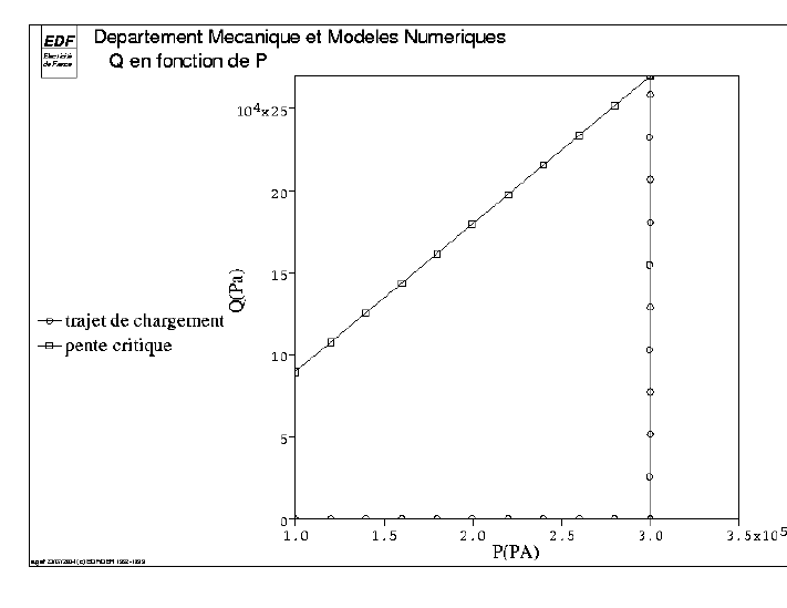
Fig. 5.2 \(Q\) based on \(P\) (B modeling).

In modeling C, vertical displacement is imposed before the hydrostatic load has reached critical pressure. The stress diverter varies over time, while the pressures on the lateral faces are kept constant. As the plasticity criterion is reached in the field of dilatance, work hardening is negative and the stress deflector decreases over time.

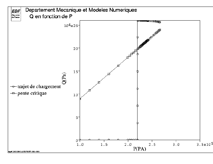
Fig. 5.3 \(Q\) based on \(P\) (C modeling).