1. Reference problem#
1.1. Geometry#
\(y\)
\({u}^{\mathit{meca}}\)
\(x\)
Figure 1.1-a: Geometry and reference problem load
It is a cylinder with height \(H=1000\mathit{mm}\), and radius \(R=1000\mathit{mm}\).
The square in bold corresponds to the axisymmetric modeling used in §3.
1.2. Material properties#
Material properties are described by the following parameters:
For thermo-metallic calculation
(\(\mathrm{16MND5}\) steel)
\(\rho {C}_{p}={5.26E}^{-3}{\mathit{J.mm}}^{-3.}°{C}^{-1}\)
\(\lambda ={33.5E}^{-3}{\mathit{W.mm}}^{-1.}°{C}^{-1}\)
Coefficient for metallurgy:
\(\mathrm{TRC}\) « standard »
\(\mathrm{AR3}=830°C\), \(\mathrm{alpha}=-0.0306\)
\(\mathrm{MS0}=400°C\), \(\mathrm{AC1}=724°C\), \(\mathrm{AC3}=846°C\)
\({\tau }_{1}=0.034\), \({\tau }_{3}=0.034\)
For thermo-metallo-mechanical calculation
Young’s module: \(E=200000\mathit{MPa}\)
Poisson’s ratio: \(\nu =0.3\)
Definition of elastic characteristics, expansion and elastic limits for modeling a material undergoing metallurgical transformations:
\({T}_{\mathrm{ref}}=20°C\)
Average thermal expansion coefficient for cold phases: \({\alpha }_{f}(T)=10{E}^{-6}\)
Average thermal expansion coefficient of the hot phase: \({\alpha }_{\gamma }(T)=10{E}^{-5}\)
Expansion coefficient definition temperature: \({T}_{\gamma }=20°C\)
Choice of the reference metallurgical phase: cold
Deformation of the non-reference phase with respect to the reference phase at temperature \({T}_{\mathrm{ref}}\): \(\Delta \varepsilon =1{E}^{-2}\)
Elastic limit of the cold phase 1 for plastic behavior:
\(\text{F\_sigm\_f}(T)=100\mathit{MPa}\)
Elastic limit of the cold phase 2 for plastic behavior:
\(\text{F\_sigm\_f}(T)=100\mathit{MPa}\)
Elastic limit of the cold phase 3 for plastic behavior:
\(\text{F\_sigm\_f}(T)=100\mathit{MPa}\)
Elastic limit of the cold phase 4 for plastic behavior:
\(\text{F\_sigm\_f}(T)=100\mathit{MPa}\)
Elastic limit of the hot phase for plastic behavior:
\(\text{F\_sigm\_f}(T)=100\mathit{MPa}\)
Function used for the mixing law on the elastic limit of multiphase material for plastic behavior:
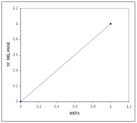
Figure 1.2-a: Law of Mixing
Definition of the 5 traction curves used in the modeling of non-linear isotropic work hardening of a material undergoing metallurgical phase changes:
Isotropic work hardening curve \(R\) as a function of the cumulative plastic deformation \(p\) for the cold phase 1
to \(20°C\):
\(p\) |
|
0.99 |
250 |
To \(120°C\):
\(p\) |
|
0.0105 |
90 |
0.032 |
160 |
0.064 |
220 |
0.1125 |
250 |
0.1815 |
270 |
Isotropic work hardening curve \(R\) as a function of the cumulative plastic deformation \(p\) for cold phase 2:
Same as previous
Isotropic work hardening curve \(R\) as a function of the cumulative plastic deformation \(p\) for cold phase 3:
Same as previous
Isotropic work hardening curve \(R\) as a function of the cumulative plastic deformation \(p\) for cold phase 4:
Same as previous
Isotropic work hardening curve \(R\) as a function of the cumulative plastic deformation \(p\) for the hot phase:
Same as previous
1.3. Boundary conditions and loads#
The base of the cylinder is stuck following \(y\):
\(\mathrm{Uy}=0\) on the base of the cylinder.
A \({u}^{\mathit{meca}}=30\mathit{mm}\) displacement is imposed on the top of the cylinder.
The temperature is imposed all over the cylinder, such that:
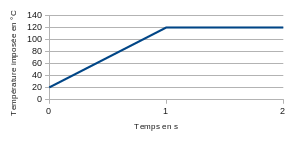
1.4. Initial conditions#
Initial temperature: \(T(x,y\mathrm{,0})=20°C\)
The following variables are initialized:
\({Z}_{f}(x,y\mathrm{,0})=0.7\)
\({Z}_{p}(x,y\mathrm{,0})=0.0\)
\({Z}_{b}(x,y\mathrm{,0})=0.3\)
\({Z}_{m}(x,y\mathrm{,0})=0.0\)
\(d(x,y\mathrm{,0})=0.0\)