1. Reference problem#
It is a cylindrical creep bar.
1.1. Geometry#
Figure 1.1-a: Geometry and reference problem load
It is a cylinder with height \(H\mathrm{=}1.0m\), and radius \(R\mathrm{=}1.0m\).
The square in bold corresponds to the axisymmetric modeling used in [§3].
1.2. Material properties#
Material properties are described by the following parameters:
For thermo-metallic calculation
(Zircaloy)
\(\rho {C}_{p}\mathrm{=}2000000{\mathit{J.m}}^{\mathrm{-}3.}°{C}^{\mathrm{-}1}\)
\(\lambda \mathrm{=}9999.9{\mathit{W.m}}^{\mathrm{-}1.}°{C}^{\mathrm{-}1}\)
Coefficient for metallurgy:
\(\mathit{teqd}\mathrm{=}809°C\), \(K\mathrm{=}1.135{E}^{\mathrm{-}2}\), \(n\mathrm{=}2.187\)
\(\mathit{t1c}\mathrm{=}831°C\), \(\mathit{t2c}\mathrm{=}0.\), \(\mathit{qsr}\mathrm{=}14614\), \(\mathit{Ac}\mathrm{=}1.58E\mathrm{-}4\)
\(m\mathrm{=}4.7\), \(\mathit{t1r}\mathrm{=}\mathrm{949,1}°C\), \(\mathit{t2e}\mathrm{=}0.\), \(\mathit{Ar}\mathrm{=}\mathrm{-}5.725\), \(\mathit{Br}\mathrm{=}0.05\)
For thermo-metallo-mechanical calculation
Young’s module: \(E\mathrm{=}200000\mathit{Pa}\)
Poisson’s ratio: \(\nu \mathrm{=}0.3\)
Definition of elastic characteristics, expansion and elastic limits for the modeling of a material undergoing metallurgical transformations:
\({T}_{\mathit{ref}}\mathrm{=}800°C\)
Average thermal expansion coefficient for cold phases: \({\alpha }_{f}(T)\mathrm{=}0\)
Average thermal expansion coefficient of the hot phase: \({\alpha }_{\gamma }(T)\mathrm{=}0\)
Expansion coefficient definition temperature: \({T}_{\gamma }\mathrm{=}800°C\)
Choice of the reference metallurgical phase: hot
Deformation of the non-reference phase with respect to the reference phase at temperature \({T}_{\mathit{ref}}\): \(\Delta \varepsilon \mathrm{=}0\)
Cold phase elasticity limit 1 for viscous behavior: \({F}_{{\mathit{sigm}}_{f}}(T)\mathrm{=}0\)
Elastic limit of the cold phase 2 for viscous behavior: \({F}_{{\mathit{sigm}}_{f}}(T)\mathrm{=}0\)
Elastic limit of the hot phase for viscous behavior: see [Figure 1.2-a]
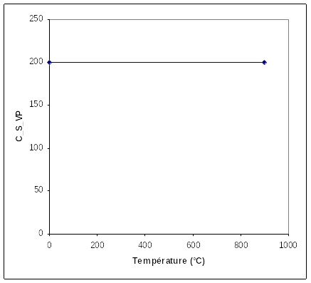
Figure 1.2.-a: Elastic limit of the hot phase for viscous behavior
Function used for the mixing law on the elastic limit of multiphase material for viscous behavior: \(f\)
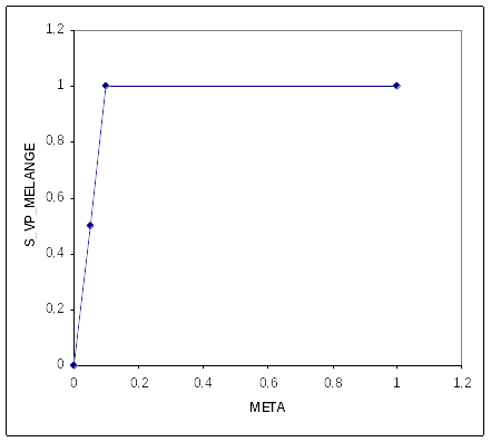
Figure 1.2-b: Law of Mixing
Definition of the work hardening modules used in modeling the phenomenon of linear isotropic work hardening of a material undergoing metallurgical phase changes:
Slope of the traction curve for cold phase 1
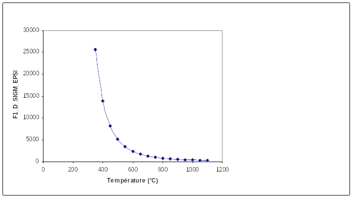
Figure 1.2-c: Tensile curve for cold phase 1
Slope of the traction curve for cold phase 2:
\(f(T)\mathrm{=}0\)
Slope of the traction curve for the hot phase:
\(f(T)\mathrm{=}0\)
Definition of the viscous parameters of the law of viscoplastic behavior taking into account metallurgy:
Parameter \(\eta\) of the viscoplastic flow law, for cold phase 1
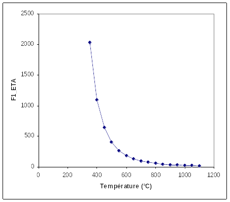
Figure 1.2-d: Parameter \(\eta\) of the viscoplastic flow law, for the cold phase 1
Parameter \(\eta\) of the viscoplastic flow law, for cold phase 2
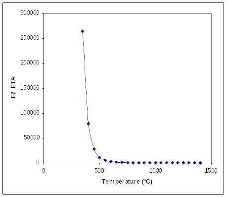
Figure 1.2-e: Parameter \(\eta\) of the viscoplastic flow law, for the cold phase 2
Parameter \(\eta\) of the viscoplastic flow law, for the hot phase:
\(f(T)\mathrm{=}0\)
Parameter \(n\) of the viscoplastic flow law, for cold phase 1:
\(f(T)\mathrm{=}5.76\)
Parameter \(n\) of the viscoplastic flow law, for cold phase 2:
\(f(T)\mathrm{=}2.94\)
Parameter \(n\) of the viscoplastic flow law, for the hot phase:
\(f(T)\mathrm{=}1.0\)
Parameter \(C\) relating to the restoration of viscous work hardening, for cold phase 1:
\(f(T)\mathrm{=}13.70539827\)
Parameter \(C\) relating to the restoration of viscous work hardening, for cold phase 2:
\(f(T)\mathrm{=}0\)
Parameter \(C\) relating to the restoration of viscous work hardening, for the hot phase:
\(f(T)\mathrm{=}0\)
Parameter \(m\) relating to the restoration of viscous work hardening, for the cold phase1:
\(f(T)\mathrm{=}5.76\)
Parameter \(m\) relating to the restoration of viscous work hardening, for the cold phase2:
\(f(T)\mathrm{=}1.0\)
Parameter \(m\) relating to the restoration of viscous work hardening, for the hot phase:
\(f(T)\mathrm{=}1.0\)
1.3. Boundary conditions and loads#
The base of the cylinder is stuck following \(y\):
\(\mathit{Uy}\mathrm{=}0\) on the base of the cylinder
A \(F\mathrm{=}25N\) traction force is imposed on the top of the cylinder
The temperature is imposed all over the cylinder for \(t\mathrm{=}\mathrm{120s}\).
\(T(x,y\mathrm{,120})\mathrm{=}800°C\)
1.4. Initial conditions#
The following variables are initialized:
\(T(x,y\mathrm{,0})\mathrm{=}800°C\)
\(\mathit{V1}(x,y\mathrm{,0})\mathrm{=}1.0\)
\(\mathit{V2}(x,y\mathrm{,0})\mathrm{=}0.0\)
\(\mathit{V3}(x,y\mathrm{,0})\mathrm{=}20.\)
\(\mathit{V4}(x,y\mathrm{,0})\mathrm{=}0.\)
\(\mathit{V1}\) : proportion of the cold phase \(\alpha\)
\(\mathit{V2}\) : proportion of the cold phase \(\alpha\) , mixed with the phase \(\beta\)
\(\mathit{V3}\) : node temperatures
\(\mathit{V4}\) : time corresponding to the temperature at which the start or end of the equilibrium transformation