1. Reference problem#
1.1. Geometry#
Drilled plates are a recurring element in the industry. The homogenization theory is well suited in such a case because of the periodicity of the bores present on the plate. The base cell is square and symmetric, we only take into account the first octant. (). For modeling A, the thickness has no influence, while this is the case for B and C. A plate thickness of 534 mm is considered.

Figure 1.1-1: Square step base cell |
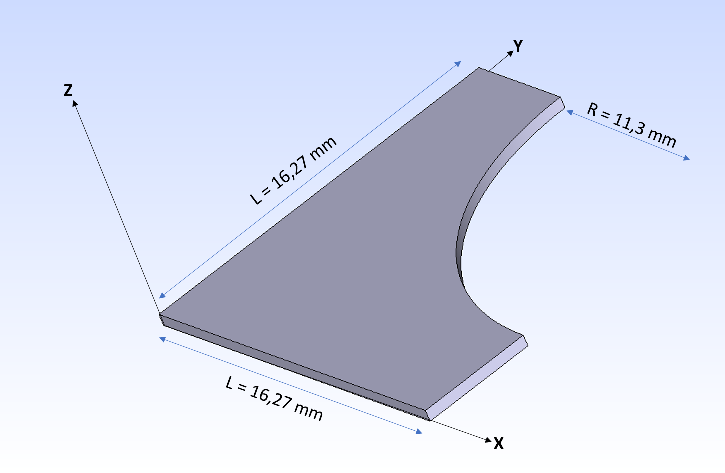
Figure 1.1-2:1/8 of the base cell |
1.2. Material properties#
Since we place ourselves in the framework of linear behavior, we choose the characteristics of the unit materials:
\(\begin{array}{c}E\text{=}1.0\mathit{MPa}\hfill \\ \mathrm{\nu }\text{=}0.3\hfill \\ k\text{=}1.0W/(m\mathrm{.}°C)\hfill \\ {C}_{p}\text{=}0J/(°C\mathrm{.}{m}^{3})\hfill \end{array}\)
1.3. Boundary conditions and loads#
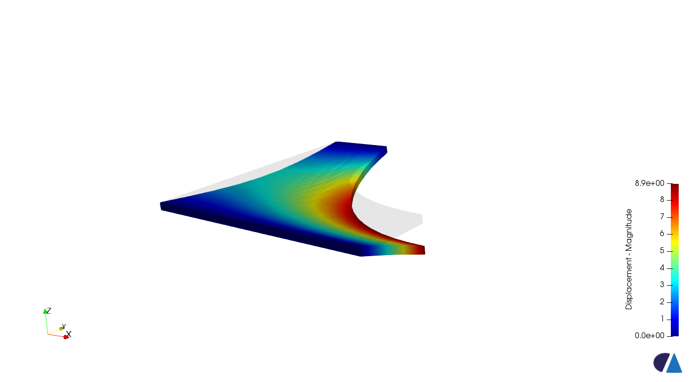
The aim is to solve six linear elasticity problems in 3D on the base cell, under periodic and symmetric boundary conditions. Each problem is associated with a \(\mathrm{\chi }\) corrector that locally accommodates \({\mathrm{\epsilon }}^{0}\) pre-deformations.
The conditions at the limits of periodicity and symmetries, for each elasticity problem, are given in the table below. The displacement associated with the problem under consideration will also be displayed.
\(y=0\to {u}_{y}=0\) on \({y}_{\mathit{min}}\) and \({y}_{\mathit{max}}\) |
\(z=0\to {u}_{z}=0\) on \({z}_{\mathit{min}}\) and \({z}_{\mathit{max}}\) |
\(y=0\to {u}_{y}=0\) on \({y}_{\mathit{min}}\) and \({y}_{\mathit{max}}\) |
\(z=0\to {u}_{z}=0\) on \({z}_{\mathit{min}}\) and \({z}_{\mathit{max}}\) |
\(y=0\to {u}_{y}=0\) on \({y}_{\mathit{min}}\) and \({y}_{\mathit{max}}\) |
\(z=0\to {u}_{z}=0\) on \({z}_{\mathit{min}}\) and \({z}_{\mathit{max}}\) |
\(y=0\to {u}_{x}={u}_{z}=0\) on \({y}_{\mathit{min}}\) and \({y}_{\mathit{max}}\) |
\(z=0\to {u}_{z}=0\) on \({z}_{\mathit{min}}\) and \({z}_{\mathit{max}}\) |
\(y=0\to {u}_{y}=0\) on \({y}_{\mathit{min}}\) and \({y}_{\mathit{max}}\) |
\(z=0\to {u}_{x}={u}_{y}=0\) on \({z}_{\mathit{min}}\) and \({z}_{\mathit{max}}\) |
\(y=0\to {u}_{x}={u}_{z}=0\) on \({y}_{\mathit{min}}\) and \({y}_{\mathit{max}}\) |
\(z=0\to {u}_{x}={u}_{y}=0\) on \({z}_{\mathit{min}}\) and \({z}_{\mathit{max}}\) |
\(z=0\to {u}_{x}={u}_{y}=0\) out of \({z}_{\mathit{min}}\) and \({z}_{\mathit{max}}\) |
|
For the linear thermal problem, the same approach is adopted as for elasticity but only three correctors are calculated.
Concealer \({\mathrm{\zeta }}^{1}\) |
|
Concealer \({\mathrm{\zeta }}^{2}\) |
|
Concealer \({\mathrm{\zeta }}^{3}\) |
|