1. Reference problem

1.1. Device description

The non-linear element is represented by the rheological model below.

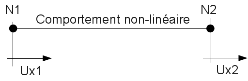
Figure 1.1-a: Device model.

The equations governing behavior are in [R5.03.17].

1.2. Modelizations

The models tested are on elements DIS_T then DIS_TR, cells SEG2 then cells POI1. The characteristics of the discrete elements are of the type: K_T_D_L, K_ TR_D_L, K_T_D_N, K_ TR_D_N.

Note: The units of the parameters must agree with the unit of effort, the unit of lengths [R5.03.17]. For all models the units are homogeneous to [N], [mm].

1.2.1. Modeling A

This modeling makes it possible to test the non-linear static cyclic behavior of the law.

1.3. Material properties

1.3.1. Modeling A

The only property is the non-linear function [R5.03.17].

The figure shows the non-linear behavior used in the test case:

• Elastic behavior up to point \((\mathrm{0.5mm},\mathrm{200.0N})\).

• Nonlinear behavior in the \(x\) local direction of the discrete, governed by the following equation:

\[\]

: label: EQ-None

R (p) =frac {{K} _ {mathit {elas}} .p} {left [1+ {left (frac {{k} _ {mathit {elas}} .p} .p} {{F} _ {u} _ {u}} — {F} _ {elas}}} .p} {{F} _ {elas}}} .p} {{F} _ {elas}} .p} {{F} _ {u}} — {F} _ {y}}right)} ^ {n}right]} ^ {(1/n)}} .p} {{F} _ {(1/n)}}

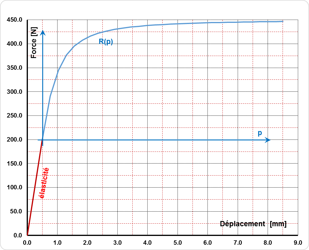
Figure 1.3.1-a : Nonlinear behavior

1.3.2. B modeling

The only property is the non-linear function [R5.03.17].

The behavior is of the « isotropic work hardening » type in the tangential plane local to the element. It is defined by the following function:

fctsy2 = DEFI_FONCTION (NOM_PARA = « DTAN »,

VALE = ( 0.0, 0.0, 0.0, 0.1, 0.1, 100.0, 0.2, 120.0, 20.2, 370.0),

)

1.3.3. C modeling

The only property is the non-linear function [R5.03.17].

The behavior is of the « kinematic work hardening » type in the tangential plane local to the element. It is defined by the following function:

fctsy2 = DEFI_FONCTION (NOM_PARA = « DTAN »,

VALE = ( 0.0, 0.0, 0.0, 0.1, 100.0, 20.1, 350.0),

)

1.4. Boundary conditions and loads

1.4.1. Modeling A

When the discrete is a SEG2, one of the nodes is blocked, on the other a displacement condition is imposed. When the discrete is a POI1 the displacement condition is imposed on this node.

The condition while traveling is a function of time:

\({U}_{0}.\mathrm{sin}(2\mathrm{\pi }.f.t)\) with \(f=1\mathit{Hz}\) and \({U}_{0}=2.0\mathit{mm}\)

1.4.2. B and C models

When the discrete is a SEG2, one of the nodes is blocked, on the other a displacement condition is imposed. When the discrete is a POI1 the displacement condition is imposed on this node.

Travel conditions are functions of time:

\(\mathit{Depl}={U}_{1.}\mathrm{sin}(2\mathrm{\pi }.{f}_{1}.t)+{U}_{2.}\mathrm{sin}(2\mathrm{\pi }.{f}_{2}.t)+{U}_{3.}\mathrm{sin}(2\mathrm{\pi }.{f}_{3}.t)\)

Following the direction \(Y\): \((u,f)=[(\mathrm{0.20,0}.80),(\mathrm{0.15,1}.50),(\mathrm{0.10,3}.00)]\)

Following the direction \(Z\): \((u,f)=[(-\mathrm{0.20,0}.90),(\mathrm{0.15,2}.00),(-\mathrm{0.10,2}.80)]\)