6. C modeling

6.1. Characteristics of modeling

Simulation at the hardware point.

6.2. Tested sizes and results

The solutions are post-processed at the single point of the model and compared to non-regression values

in terms of isotropic effective pressure \(P\text{'}\), with:

\(P\text{'}=\frac{1}{3}\mathit{tr}(\mathrm{\sigma }\text{'})\)

Identification	Reference type	Reference value	Tolerance
\(t=70.s\)	“AUTRE_ASTER”	167597.Pa	%
\(t=\mathrm{91,15}s\)	“AUTRE_ASTER”	Not	%
\(t=\mathrm{99,3}s\)	“AUTRE_ASTER”	Not	%

And deviatoric constraint \(Q\), with:

\(Q={\mathrm{\sigma }}_{\mathit{zz}}-{\mathrm{\sigma }}_{\mathit{xx}}\)

Identification	Reference type	Reference value	Tolerance
\(t=70.s\)	“AUTRE_ASTER”	110000.Pa	%
\(t=\mathrm{91,15}s\)	“AUTRE_ASTER”	-69201. Not	%
\(t=\mathrm{99,3}s\)	“AUTRE_ASTER”	Not	%

6.3. notes

The purpose of this modeling is to treat the passage of the instability line in the case of loose sand. In fact, the constraint deviator \(Q\) has a maximum on this line whose value is less than the imposed maximum stress setpoint \({Q}_{\mathit{max}}=110\mathit{kPa}\). Consequently, the stress control of the test is not possible at this location, and generally leads either to a discrepancy in the calculation, or to a false result that is perfectly unstable (very significant jump in stress and deformation, see the red curve in the Figure). The calculation of the exact solution involves switching the test to controlled deformation when instability is detected (blue curve).

line of instability

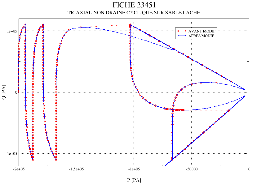
Figure 6.3-1: Comparison of the solution under controlled stress (red) and under controlled deformation (blue) when crossing the instability line