3. Modeling A

3.1. Characteristics of modeling

This is a D_ PLAN modeling using linear HM- XFEM elements.

3.2. Characteristics of the mesh

The square on which the modeling is performed is divided into 16 QUAD4. The interface is unmeshed and cuts the square horizontally. The mesh is shown in Figure.

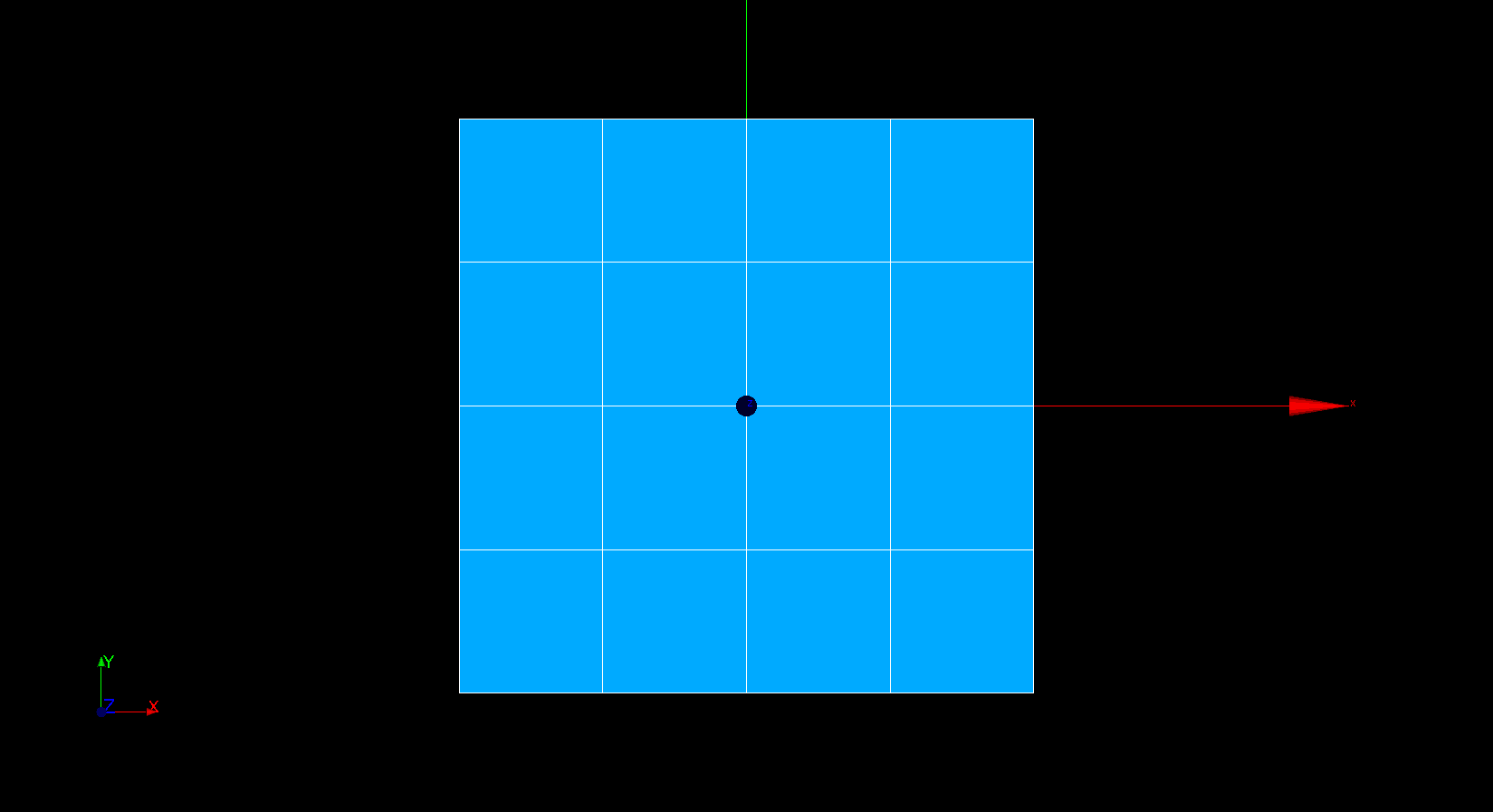
Figure 3.2-a : 2D mesh

3.3. Tested sizes and results

The results are obtained with*Code_Aster* (resolution with STAT_NON_LINE). We test the horizontal stress \({\sigma }_{\mathit{xx}}\), which is assumed to be uniformly zero, and the vertical stress \({\sigma }_{\mathit{yy}}\), which is assumed to be uniform, with a value of \(-E\). To do this, we test MIN and MAX of these two sizes throughout the element. The results obtained are summarised in the table below.

Tested quantities	Reference type	Reference values	Tolerance
SIGMAXX (MPa) MIN	“ANALYTIQUE”	0.0	30
SIGMAXX (MPa) MAX	“ANALYTIQUE”	0.0	45
SIGMAYY (MPa) MIN	“ANALYTIQUE”	-5800.0	8%
SIGMAYY (MPa) MAX	“ANALYTIQUE”	-5800.0	4%

The movements following \(y\) and the deformation are shown in Figure. A linear compression of the square is clearly observed, which is little disturbed by the presence of the crack.

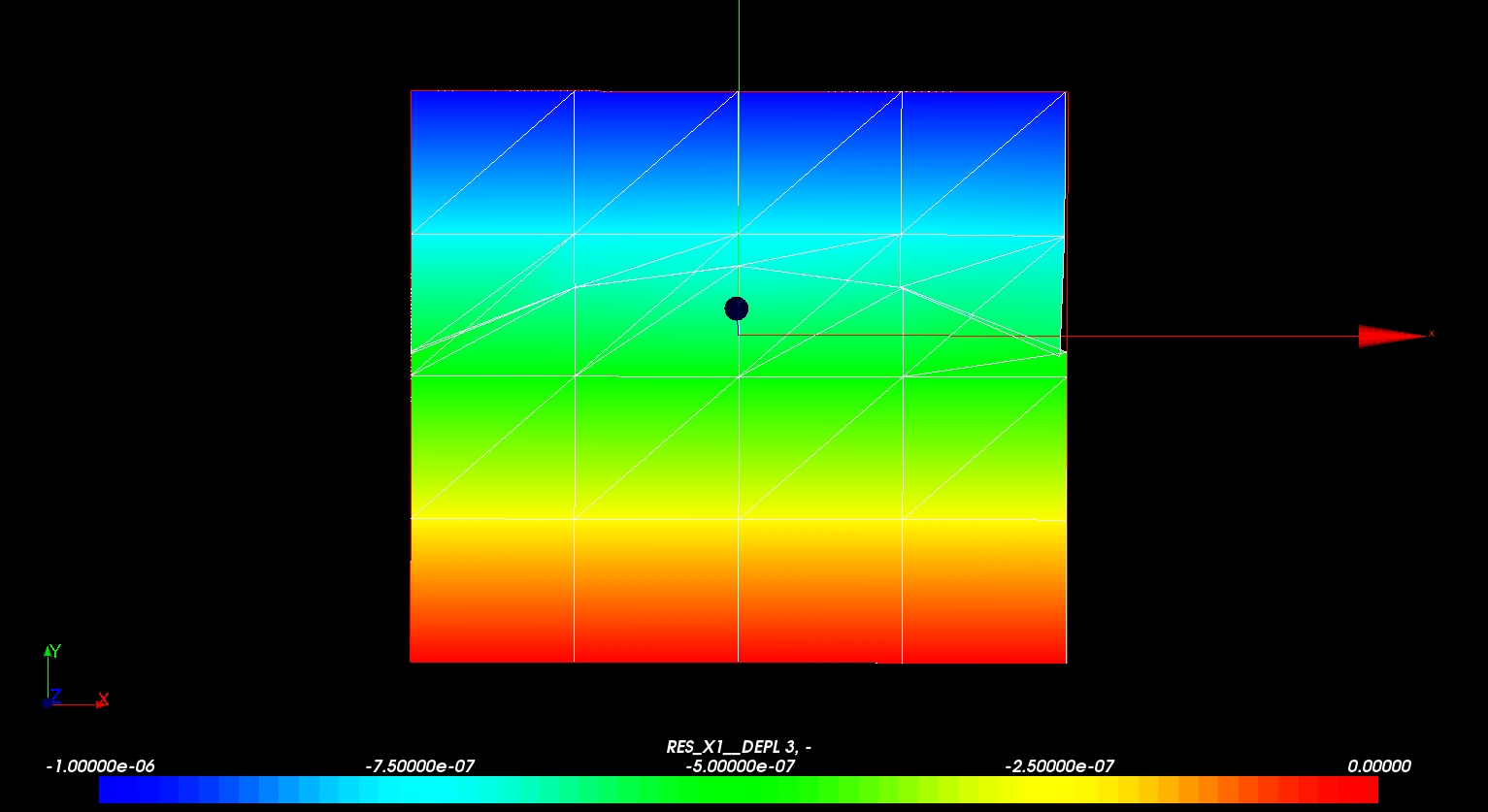
Figure 3.3-a : Field of movement by direction (Oy)

On the other hand, in Figures and, the differences in the stress field with respect to the analytical solution are observed, in particular in the vicinity of the crack and near the edges. The relative precision obtained may seem mediocre but it must be related to the small number of elements used and the significant curvature of the discontinuity.

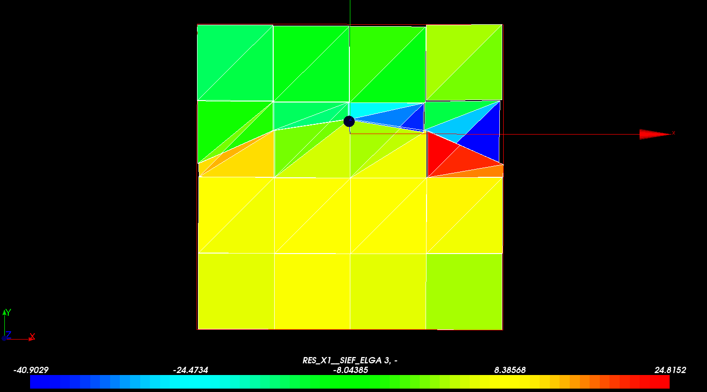
Figure 3.3-b : Constraint field sxx

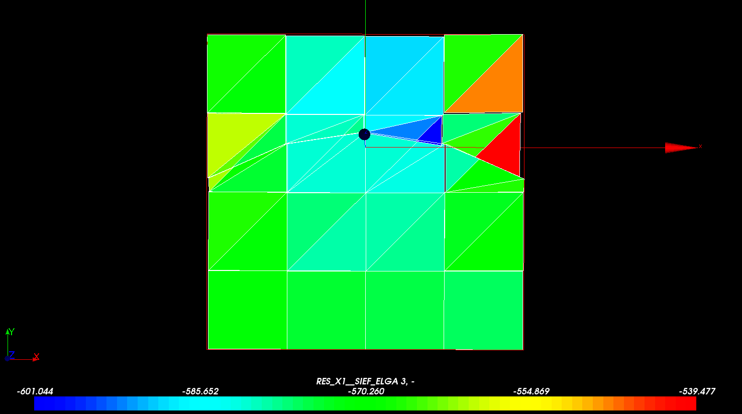
Figure 3.3-c : Constraint field syy