5. C modeling#
In this modeling, a grid in quadrangles is produced, with refinement near the contact zone.
5.1. TP implementation#
5.1.1. Realization of geometry#
In this modeling, we must partition the geometry so that it can be meshed into quadrangles.
In module GEOM, an illustration of the possible partition is given in the figure:
Take face \(\mathit{SPHHAU}\) and explain all its points (New Entity → Explode: Vertex menu), then we get the 4 points \(A2\), \(B2\), \(C2\) and \(D2\)
Create the points \(M\), \(N\) and \(P\) in order to generate the red partition lines (New Entity → Basic → Point menu): \((\mathrm{0,}\mathrm{25,}0)\), \((\mathrm{25,}\mathrm{25,}0)\) and \((\mathrm{25,}\mathrm{50,}0)\)
Generate partition lines (New Entity → Basic → Line menu)
Partition \(\mathit{SPHHAU}\) with the lines above (Menu Operations → Partition).
By symmetry, you can generate a new lower face (Menu Operations → Transformation → Mirror Image) by choosing the X axis to achieve the symmetry
It remains to assemble the two new spheres to form a single object GEOM (Menu New Entity → Build → Compound*) *.
Define all groups as in modeling A, which will be needed to assign boundary conditions and loads (New Entity → Group → Create Group menu)
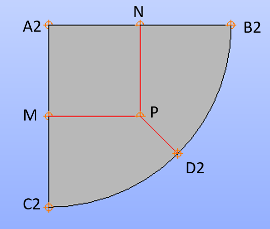
Figure 5.1: Top disk partition
5.1.2. Realization of the mesh#
For the mesh, we choose to refine around the contact zone using a geometric progression on the circumference and on the radius. It may be necessary to reorient some segments in the Mesh module:
The mesh is defined by the menu Mesh→ Create Mesh with the geometry to be meshed. The mesh will be carried out in triangles, and the automatic meshing hypotheses « Assign a set of hypotheses →2D: Automatic Quadrangulation » will be used by choosing the number of segments 15. We calculate the mesh (Menumesh → Compute).
We define sub-mesh (Menumesh → Create Sub-mesh) with groups \(\mathit{CONT}1\) and \(\mathit{CONT}2\). It is carried out using the Wire Discretization algorithm, the Start and End Length hypothesis (for example, 0.2mm and 2.0mm) and the advanced hypothesis Propagation of Node Distribution on Opposite Edges. A linear mesh containing approximately 3500 quadrangles and 4000 nodes is then obtained.
Change the mesh from linear to quadratic: « Modification -> Convert to/from quadratic ».
We will then import the groups from the geometry (Menu Mesh → Create Groups from Geometry).
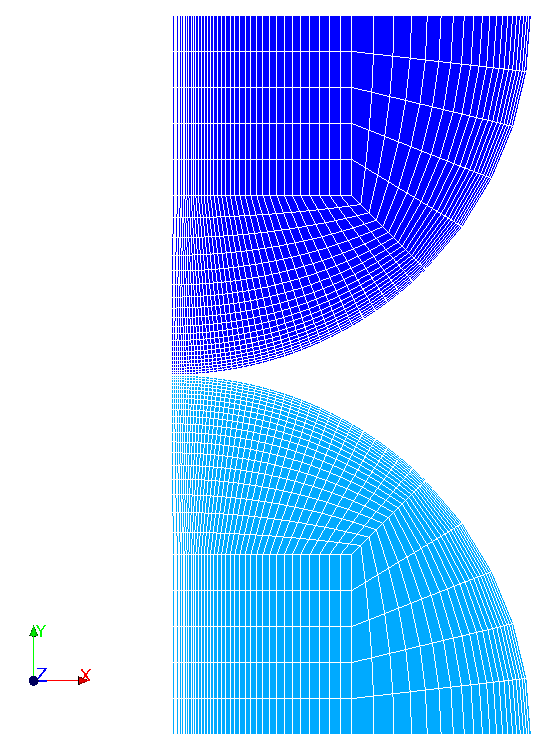
Figure 5.2: Quadrangle mesh obtained for C modeling
5.2. Tested sizes and results#
Identification |
Reference type |
Reference value |
Tolerance |
\({\sigma }_{\mathit{yy}}\) point \(\mathit{C1}\) |
“ANALYTIQUE” |
\(\mathrm{-}\mathrm{2798,3}\mathit{Mpa}\) |
|