2. Reference solution#

2.1. Calculation method#

The analytical reference solution is given by:

(2.1)#\[\begin{split} \ begin {array} {ccc}\ mathit {Ux} &\ text {=} & 0.2\ mathrm {\ times} {Z} ^ {2}\ mathrm {\ times} X\ mathrm {\ times} X\ mathrm {\ times}} Y\\\ times} Y\\\ mathit {Uy} &\ text {=} & 0.2\ mathrm {\ times} {Z} ^ {2}\ mathrm {\ times} {2}\ mathrm {\ times} X\ mathrm {\ times} Y\\\ mathit {Uz} &\ text {=} &\ mathrm {-} 0.2\ mathrm {\ times} (1. + {X} ^ {2} + {Y} ^ {2})\ mathrm {\ times} (1+0.01\ mathrm {\ times} Z)\ mathrm {-} 0.01\ mathrm {\ ast}})\ mathrm {\ ast}))\ mathrm {\ times} (1+0.01\ mathrm {-} Z)\ mathrm {-} 0.01\ mathrm {-} 0.01\ mathrm {\ ast}} Z\ mathrm {-} 0.3\ end {array}\end{split}\]

The Dirichlet and Neumann conditions and the source term are obtained by the method of manufactured solutions [bib1].

We start by determining the gradient of transformation \(\underline{\underline{F}}\):

(2.2)#\[ \ underline {\ underline {F}} =\ underline {\nabla}\ underline {U} +\ underline {\ underline {\ underline {\ mathrm {Id}}}}\]

Knowing the normal \(\underline{N}={[\mathrm{0,}\mathrm{0,}-1]}^{T}\) to the surface \(\text{ESCLAVE}\) in the undeformed configuration, we obtain its expression in the deformed configuration by the Nanson formula:

\[\]

: label: eq-4

underline {n} =frac {{underline {underline {underline {F}}}} ^ {-T}underline {N}} {parallel {underline {F}}}}} ^ {-T}underline {N}parallel}

Knowing the Hooke tensor \(\underline{\underline{\underline{\underline{A}}}}\) and the Green-Lagrange tensor \(\underline{\underline{E}}\) and the Green-Lagrange tensor, we calculate the second Piola-Kirchhoff tensor \(\underline{\underline{S}}\):

\[\]

: label: eq-5

underline {underline {E}} =frac {1} {2} ({underline {underline {F}}}}} ^ {T}cdotunderline {underline {F}}} -underline {underline {F}}} -underline {underline {underline {F}}} -underline {underline {F}}} -underline {underline {F}}} -underline {underline {F}}} -underline {underline {F}}})

(2.3)#\[ \ underline {\ underline {S}} =\ underline {\ underline {\ underline {\ underline {A}}}}}:\ underline {\ underline {E}}}:\ underline {\ underline {E}}}\]

It should be noted that the second Piola-Kirchhoff tensor \(\underline{\underline{S}}\) makes it possible to obtain forces in an undeformed configuration per unit of undeformed area:

(2.4)#\[ \ frac {d\ underline {{f} _ {0}}}} {\ mathrm {dA}} =\ underline {\ underline {S}}}\ cdot\ underline {N}\]

As we are looking to determine forces in a deformed configuration, we will determine the first Piola-Kirchhoff tensor \(\underline{\underline{\Pi }}\)

(2.5)#\[ \ underline {\ underline {\ Pi}} =\ underline {\ underline {F}}\ cdot\ underline {\ underline {S}}\]

We can thus determine volume forces \({\underline{f}}_{\mathrm{vol}}\):

(2.6)#\[ {\ underline {f}} _ {\ mathrm {vol}}} =\ text {-div}\ underline {\ underline {\ pi}}\]

Knowing the normal in initial configuration on the various faces and the first Piola-Kirchhoff \(\underline{\underline{\Pi }}\) tensor, we can calculate the surface forces in deformed configuration:

(2.7)#\[ {\ underline {f}} _ {\ text {surf}} =\ underline {\ underline {\ Pi}}\ cdot\ underline {N}}\]

On the surface \(\text{BAS}\) that is in contact, a particular treatment is needed. In fact, normal forces are taken into account by contact:

(2.8)#\[\begin{split} \ begin {array} {ccccc} {\ underline {f}}} _ {\ text {surf}} _ {\ text {surf}}} ^ {\ text {BAS}} & {\ underline {f}} _ {{\ text {surf}}} _ {n}} _ {n}} _ {n}} _ {n}} _ {n}} ^ {\ text {surf}} _ {n}} ^ {\ text {surf}}} _ {n}} ^ {\ text {surf}}} ^ {\ text {BAS}}\\ &\ text {=}} & {\ underline {f}}} _ {\ text {contact}} & +& {\ underline {f}} _ {{\ text {surf}}} _ {t}} _ {t}} _ {t}} _ {t}}} _ {\ text {f}} _ {\ text {f}} _ {\ text {f}} _ {\ text {surf}}} _ {\ text {surf}}} _ {\ text {surf}}} _ {\ text {surf}}} _ {\ text {surf}}} _ {\ text {surf}}} _ {\ text {surf}}} _ {\ text {surf}}} _ {\ text {surf}}} _ {\ text {surf}}} _ {{\ text {surf}}} _ {t}}} ^ {\ text {BAS}}\ end {array} BAS BAS\end{split}\]

Where \(p\) refers to contact pressure. It can be determined by the expression:

(2.9)#\[ p= (\ underline {\ underline {\ Pi}}}\ cdot\ underline {N})\ cdot\ underline {n}\]

Therefore, only tangential forces should be applied. They are calculated by the expression:

(2.10)#\[\begin{split} \ begin {array} {ccc} {\ underline {f}}} _ {{\ text {f}}} _ {t}} ^ {\ text {BAS}} &\ text {=} & {\ underline {f}}} _ {\ text {f}}} _ {\ text {f}}} _ {\ underline {f}} _ {\ text {surf}}} _ {n}}} _ {n}} ^ {n}} ^ {\ text {BAS}}\\ &\ text {=}} & {\ underline {f}}} _ {\ text {surf}} ^ {\ text {BAS}} - ({\ underline {f}}} _ {{\ text {surf}}} _ {\ text {surf}}} _ {n}} _ {n}} _ {n}} _ {n}} _ {n}} _ {\ text {surf}} _ {\ text {surf}}} _ {\ text {surf}} _ {\ text {surf}}} _ {\ text {surf}}} _ {\ text {surf}}} _ {\ text {surf}} _ {\ text {surf}}} _ {\ text {surf}}} _ {\ text {surf}}} _ {BAS BAS\end{split}\]

Regarding contact efforts, it is absolutely essential to build the manufactured solution in such a way that they verify the contact equations [bib2], namely:

(2.11)#\[\begin{split} \ begin {array} {ccc}\ text {gap} (\ underline {U}) &\ text {}\ ge\ text {} & 0\ p&\ text {}\ le\ text {}\ le\ text {} & 0\\ p\ cdot\ cdot\ cdot\ cdot\ cdot\ text {gap} (\ underline {U}) (\ underline {U}) &\ text {=} & 0\ end {array} & 0\ end {array}\end{split}\]

This verification is done after analytically calculating the pressure and the displacement jump associated with the manufactured solution, in general with a formal calculation tool (in this case, it is the Python module sympy). We must then visualize them, in order to check retrospectively that the solution we have built does indeed verify (). In the case of this test, we have represented analytical pressure and displacement jumps in figures and. We notice that they verify \(p<0\) and \(\text{gap}(\underline{U})=0\), which is characteristic of a fully contacting surface, and in accordance with ().

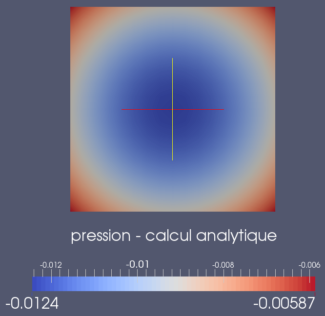
Figure 2.1-1: Validity of the manufactured solution: pressure p

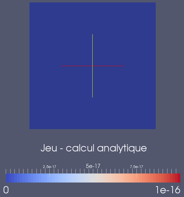
Figure 2.1-2: Validity of the manufactured solution: Gap game (U)

2.2. Reference quantities and results#

The value of the difference between analytical solutions and calculated on the mesh: \(\sum ^{\text{noeuds}n}\mid {\underline{U}}_{\text{n}}^{\text{calc}}-{\underline{U}}_{\text{n}}^{\text{ref}}\mid\) and \(\sum ^{\text{noeuds}n}\mid {p}_{\text{n}}^{\text{calc}}-{p}_{\text{n}}^{\text{ref}}\mid\).

In the case of models that perform a convergence analysis with the fineness of the mesh, the speed of convergence with the fineness of the mesh from the calculated solution to the analytical solution in standard \({L}_{2}\):

the largest real \({\alpha }_{U}>0\) such as \({\parallel {\underline{U}}^{\text{calc}}-{\underline{U}}^{\text{ref}}\parallel }_{\mathrm{0,}\Omega }<{C}_{U}\times {h}^{{\alpha }_{U}}\) where \({C}_{U}\) is independent of \(h\) for displacement;
the largest real \({\alpha }_{p}>0\) such as \({\parallel {p}^{\text{calc}}-{p}^{\text{ref}}\parallel }_{\mathrm{0,}{\Gamma }_{C}}<{C}_{p}\times {h}^{{\alpha }_{p}}\) where \({C}_{p}\) is independent of \(h\) for contact pressure.

2.3. Uncertainty about the solution#

None

2.4. Bibliographical references#

Document U2.08.08, Using the Manufactured Solutions Method for Software Validation, Code_Aster U2 Documentation
r5.03.50 Discreet formulation of contact friction r5.03.50 Discreet formulation of contact friction r5.03.50 Discreet formulation of contact friction