1. Reference problem#
1.1. Geometry#
We consider an element as a material point.
1.2. Material properties#
1.2.1. Hujeux and Iwan models of behavior#
The isotropic elastic properties of the material are \(E=619.33\) MPa and \(\nu =0.3\).
The anelastic parameters specific to the Hujeux model (modeling A) are:
\(n=0.4\), \(\mathrm{\beta }=24\), \(b=0.2\), \(d=2.5\).
\(\mathrm{\varphi }=33°\), \(\mathrm{\psi }=33°\), \({P}_{c0}=-1\) MPa, \({P}_{\mathit{ref}}=-1\) MPa
\({a}_{\mathit{cyc}}=1\times10^{-4}\), \({a}_{\mathit{mon}}=8\times10^{-3}\)
\({c}_{\mathit{cyc}}=1\times10^{-1}\), \({c}_{\mathit{mon}}=2\times10^{-1}\)
\({r}_{\mathit{ela}}^{d}=5\times10^{-3}\), \({r}_{\mathit{ela}}^{i}=1\times10^{-3}\), \({r}_{\mathit{ela}}^{d,c}=5\times10^{-3}\), \({r}_{\mathit{ela}}^{i,c}=1\times10^{-3}\)
\({r}_{\mathit{hys}}=5\times10^{-2}\), \({r}_{\mathit{mob}}=9\times10^{-1}\)
\({x}_{m}=1\), \(\alpha=1\)
The anelastic parameters of the Iwan model (modeling B) are for their part \(\gamma_{\mathrm{ref}}=2\times10^{-4}\) and \(n=0.78\).

Fig. 1.1 Predictions of the secant shear modulus normalized with distortion by Hujeux and Iwan models.#

Fig. 1.2 Predictions of reduced damping with distortion by Hujeux and Iwan models.#
1.2.2. Behaviour model CSSM#
The parameters specific to the model CSSM [r7.01.44] are grouped together in the Section 1.3 concerning the C modeling.
1.3. Boundary conditions and loads#
As a reminder, the use of the SIMU_POINT_MAT command makes it possible to directly impose a field of deformations and/or constraints.
A zero evolution during loading is imposed for the following components of the stress and strain tensors:
\({\mathrm{d}\sigma}_{xx}={\mathrm{d}\sigma}_{yy}={\mathrm{d}\sigma}_{zz}=0\)
\({\mathrm{d}\varepsilon}_{yz}={\mathrm{d}\varepsilon}_{zx}=0\)
The evolution of Fig. 1.3 is imposed for \(\varepsilon_{xy}\) shear deformations:
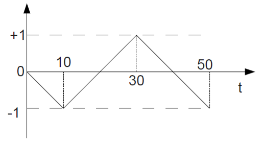
Fig. 1.3 Imposed loading chronology for the \(\varepsilon_{xy}\) (standardized) deformation component.#
Several calculations are carried out by varying the amplitude of deformations according to the values \(\left\{2\times10^{-5},2\times10^{-4},2\times10^{-3}\right\}\).
1.4. Initial conditions#
The initial stress state is isotropic and corresponds to a pressure equal to \(50\) kPa.